The NASA C-MAPSS PHM08 Prognostics Challenge was first introduced at the 2008 Prognostics and Health Management Conference to address the scarcity of run-to-failure data. It has become a widely recognized academic benchmark for predictive maintenance modeling.

To this day, run-to-failure data remains scarce for two main reasons. Collecting data from production-grade assemblies like jet engines all the way to failure takes a long time and offers incumbents who retain their proprietary data a competitive advantage, allowing them to build their own state-of-the-art predictive maintenance models first.

This dataset is a bit of a compromise; while it helps fill in the gap of lacking aerospace RUL data, it does so through synthetically generated data. In order to create this dataset without waiting for hundreds of real multimillion-dollar jet engines to have a catastrophic failure, NASA turned to MATLAB and Simulink. These graphical programming environments are commonly used for modeling, simulating, and analyzing multi-domain dynamical systems. In this particular case, they were used to generate the sensor data and degradation trends present in the C-MAPSS datasets.

While synthetic data may not accurately capture all of the intricate complexities during a real turbofan jet engine’s operation, it still presents a uniquely valuable, experimental environment for testing various approaches to machine learning for health management.

In this project, I gave myself the task of seeing how far I can take gradient boosting models on this dataset, especially when compared to deep learning alternatives. You can view the interactive web app at https://z-tempest.github.io/JetBoost/

Initial Exploration

C-MAPSS is composed of four datasets:

Subset	Operating conditions	Fault modes	Train / test engines
FD001	1	1 (HPC)	100 / 100
FD002	6	1 (HPC)	260 / 259
FD003	1	2 (HPC + fan)	100 / 100
FD004	6	2 (HPC + fan)	249 / 248

During exploratory data analysis, sensor value correlation matrices were visualized for each dataset and its individual operating conditions. All datasets with a single operating condition possessed several indeterminate sensor-correlation relationships (Figure 1).

Figure 1

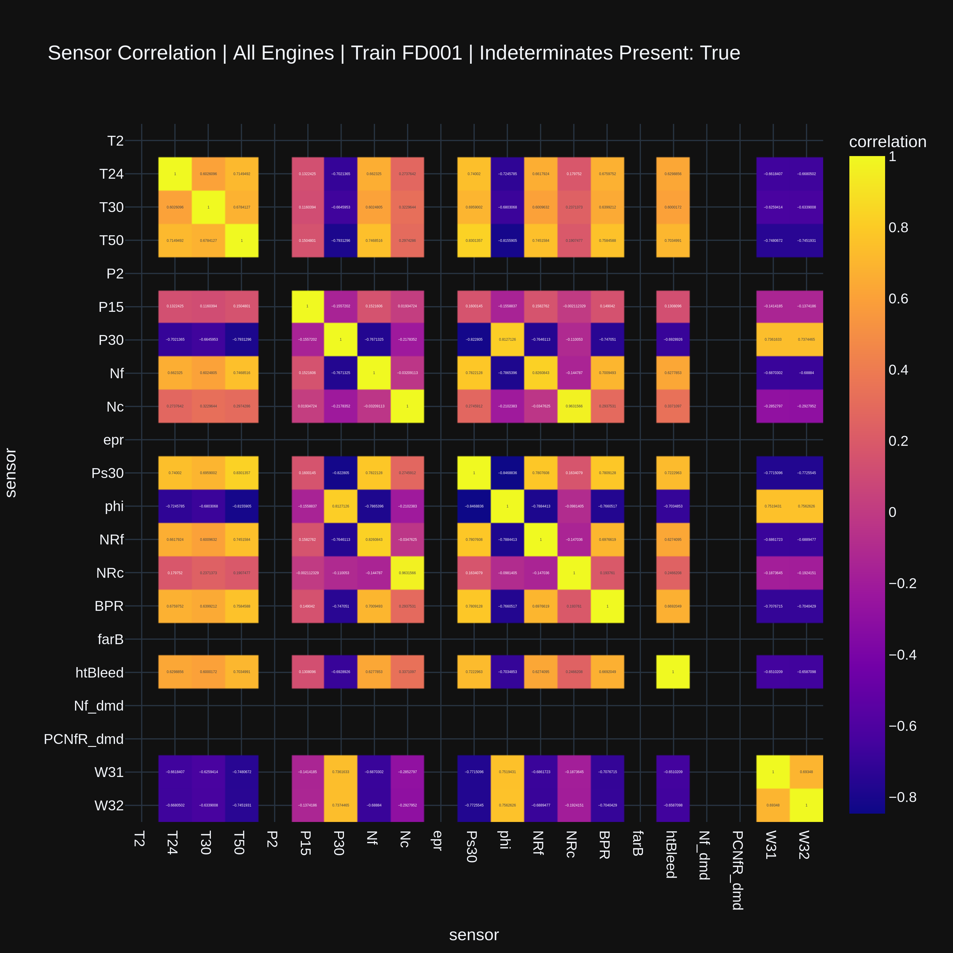
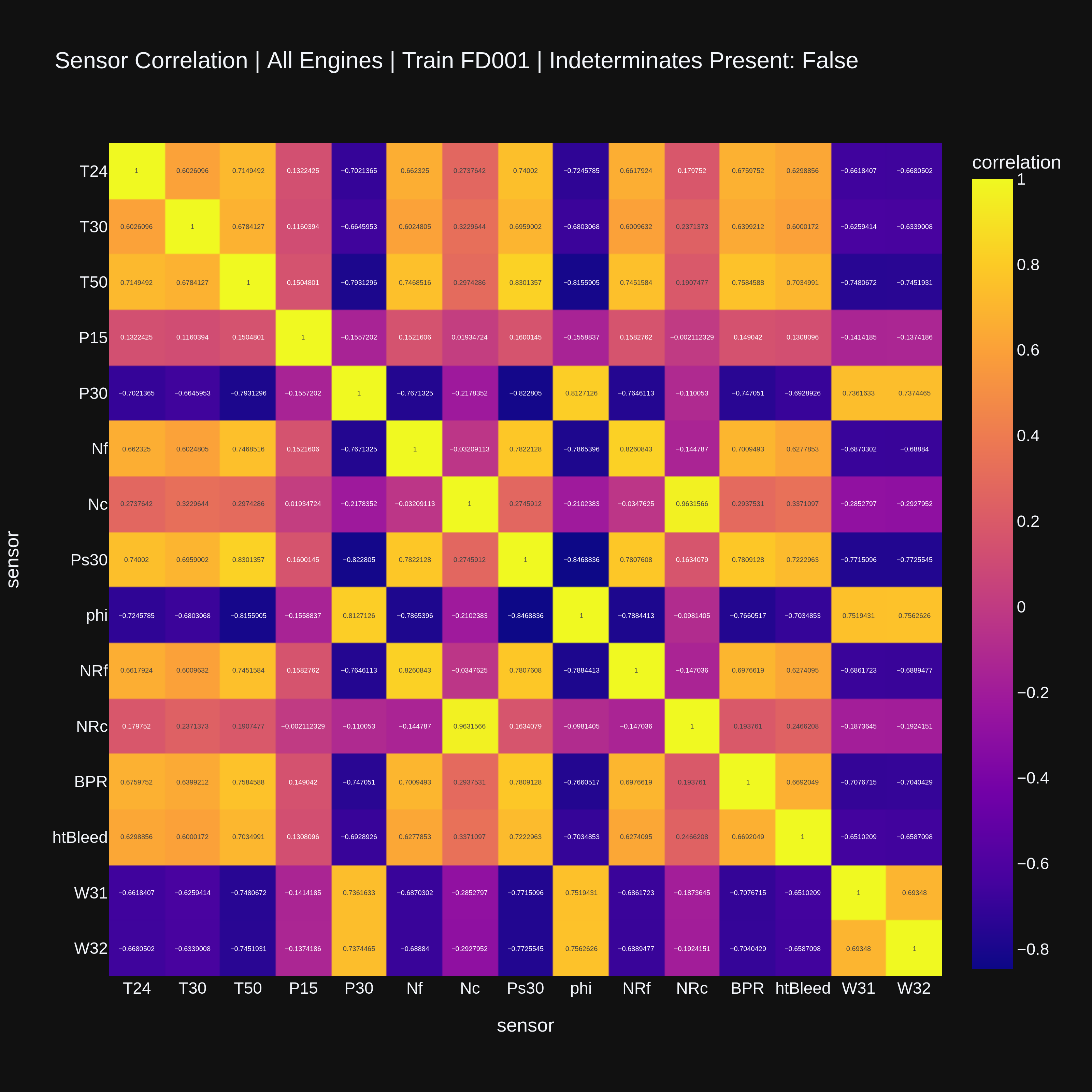
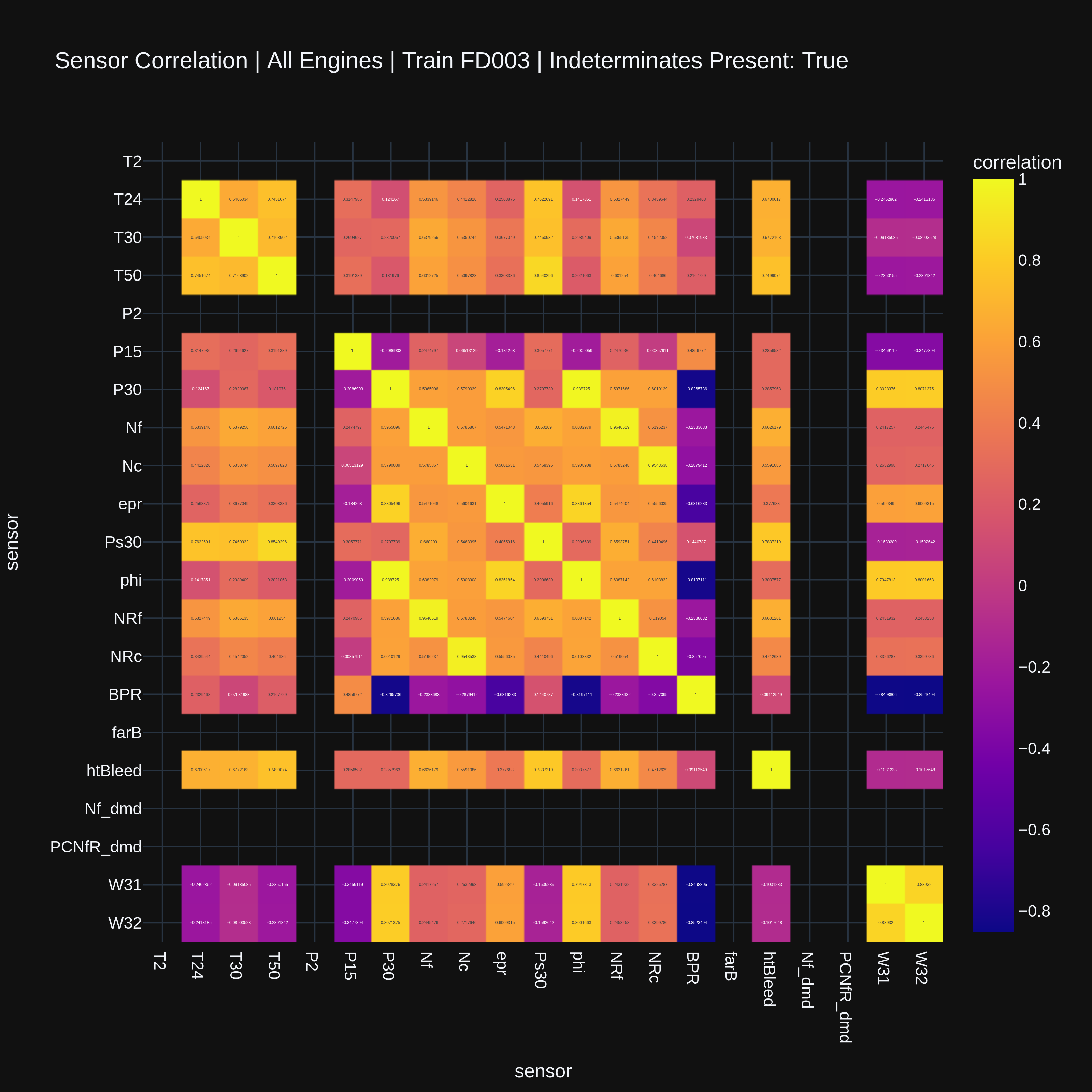
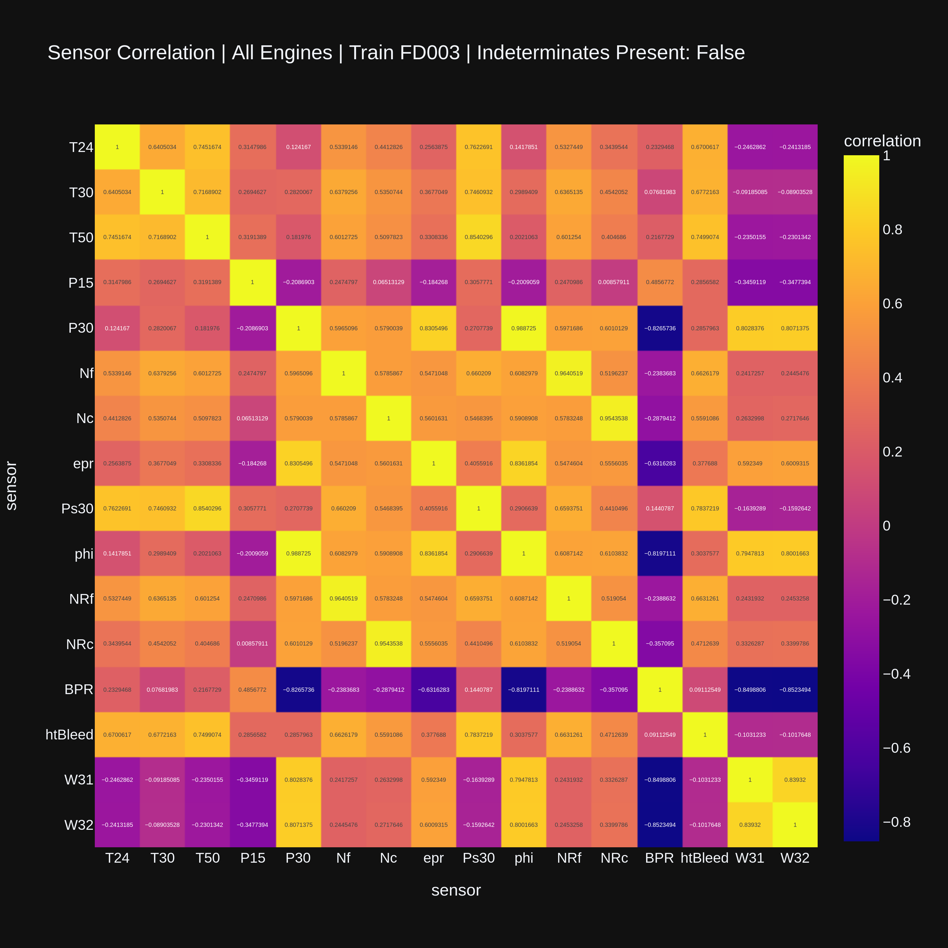
When visualizing datasets with multiple operating conditions, such as FD002 and FD004, these indeterminate sensor-correlation relationships were not displayed (Figure 2).

Figure 2

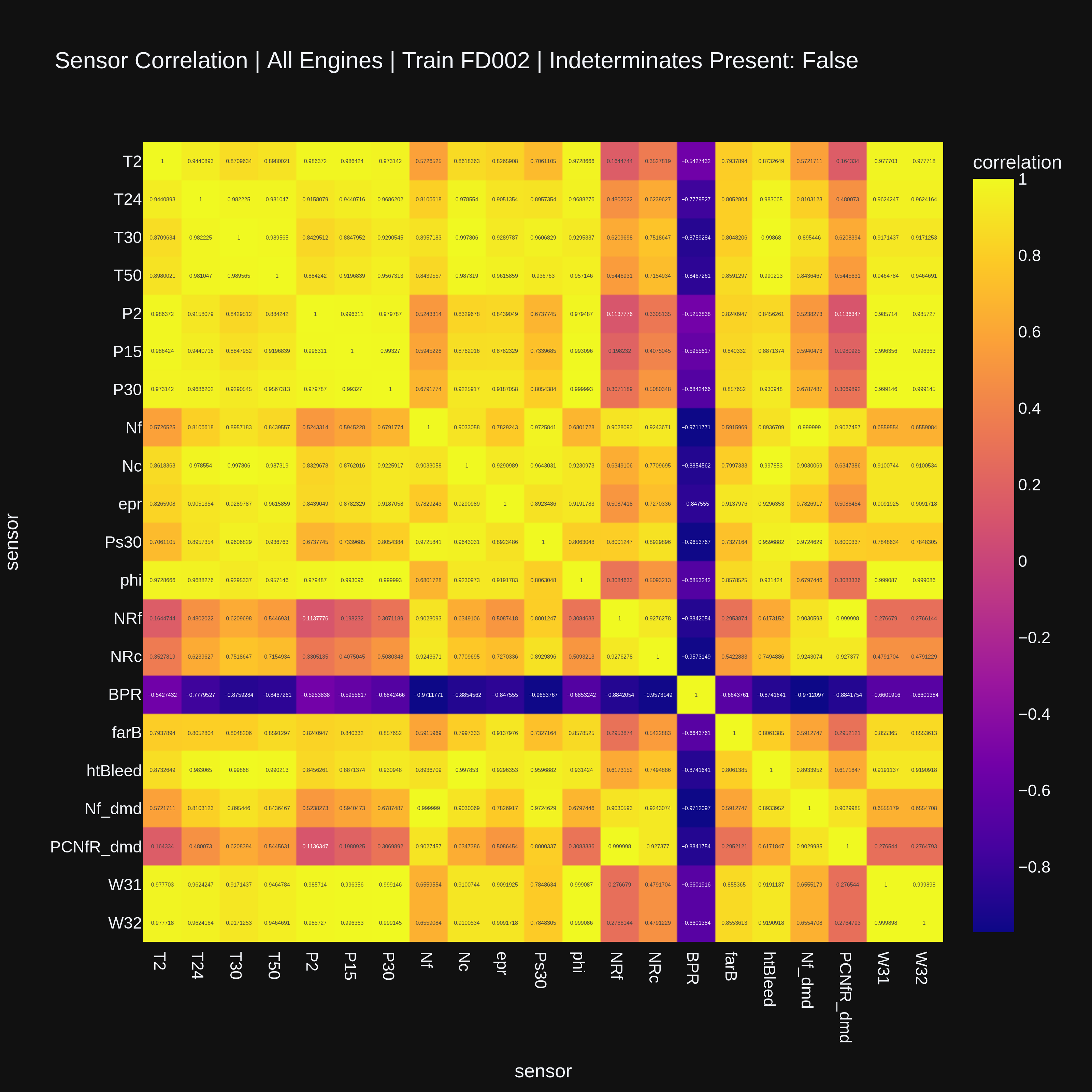
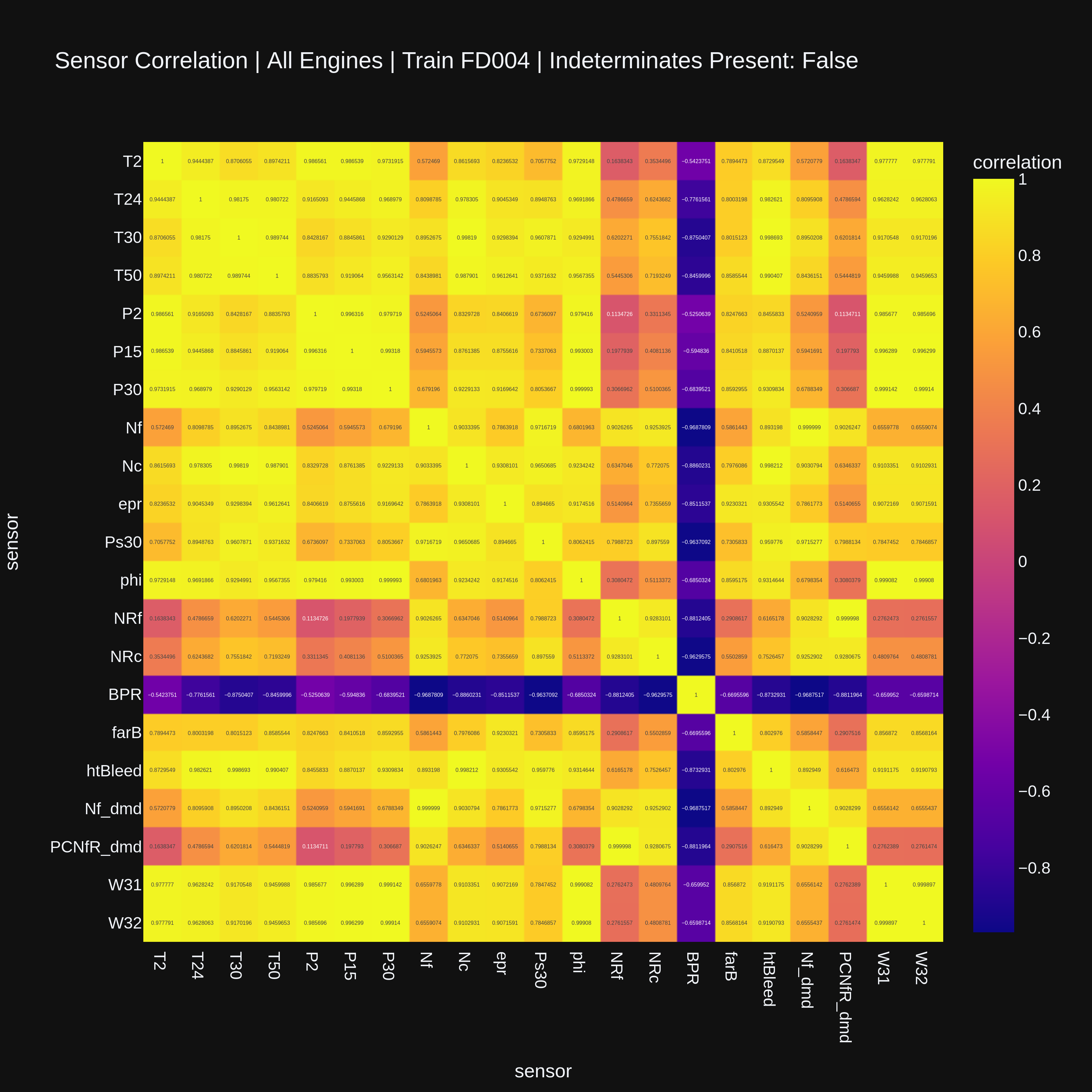
After computing the sensor correlation matrices of FD002 and FD004 under partitioned operating conditions, the indeterminate relationships returned (Figure 3).

Figure 3

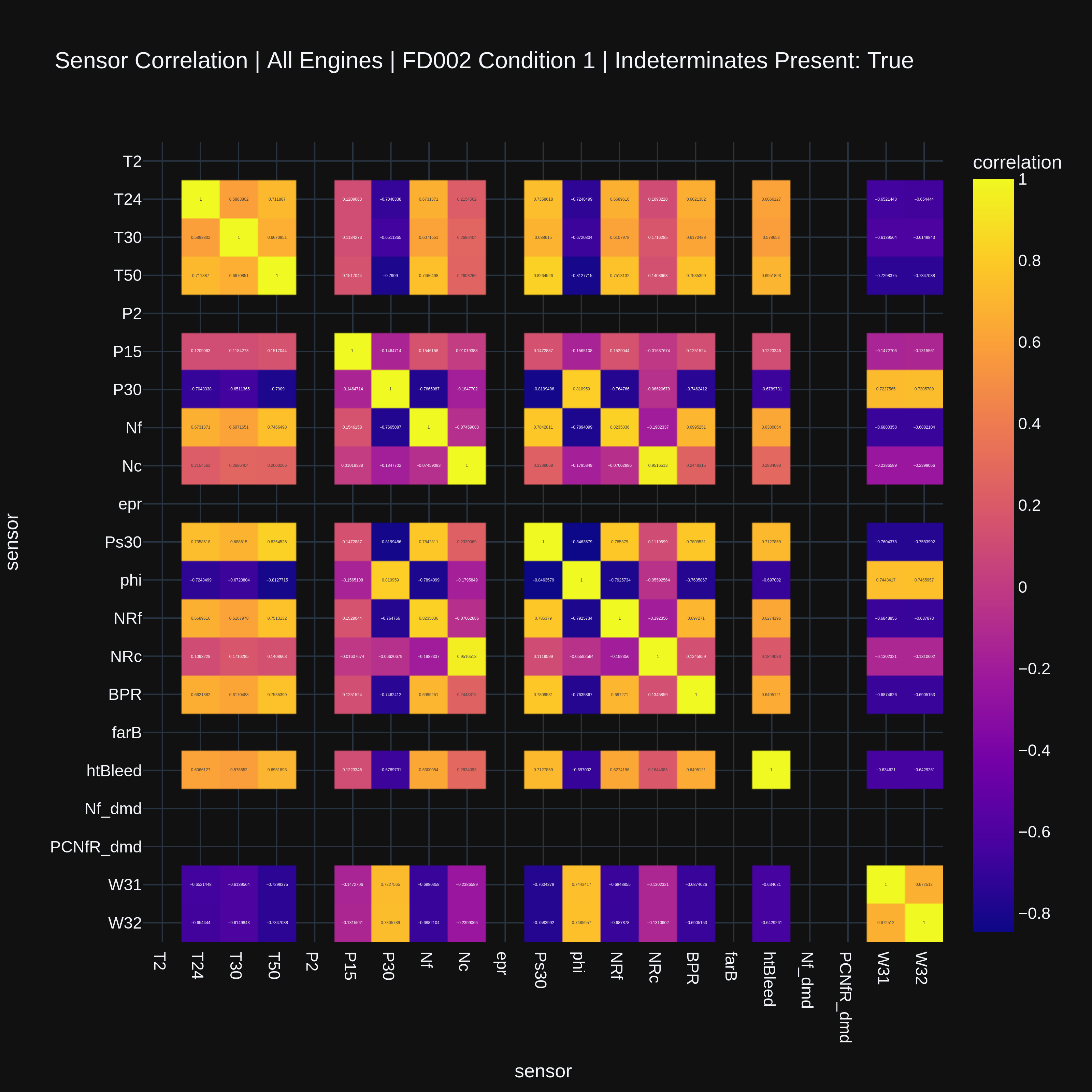
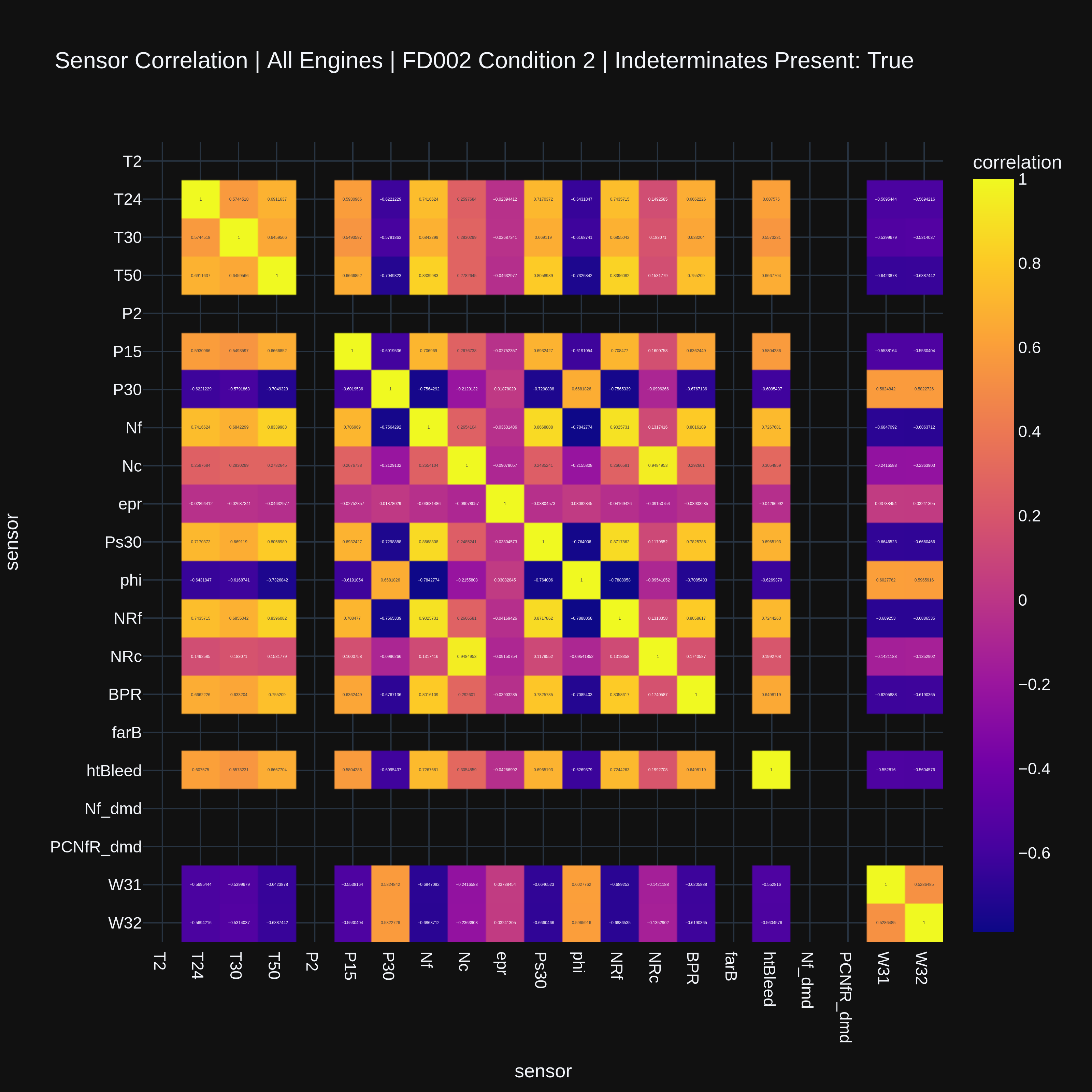
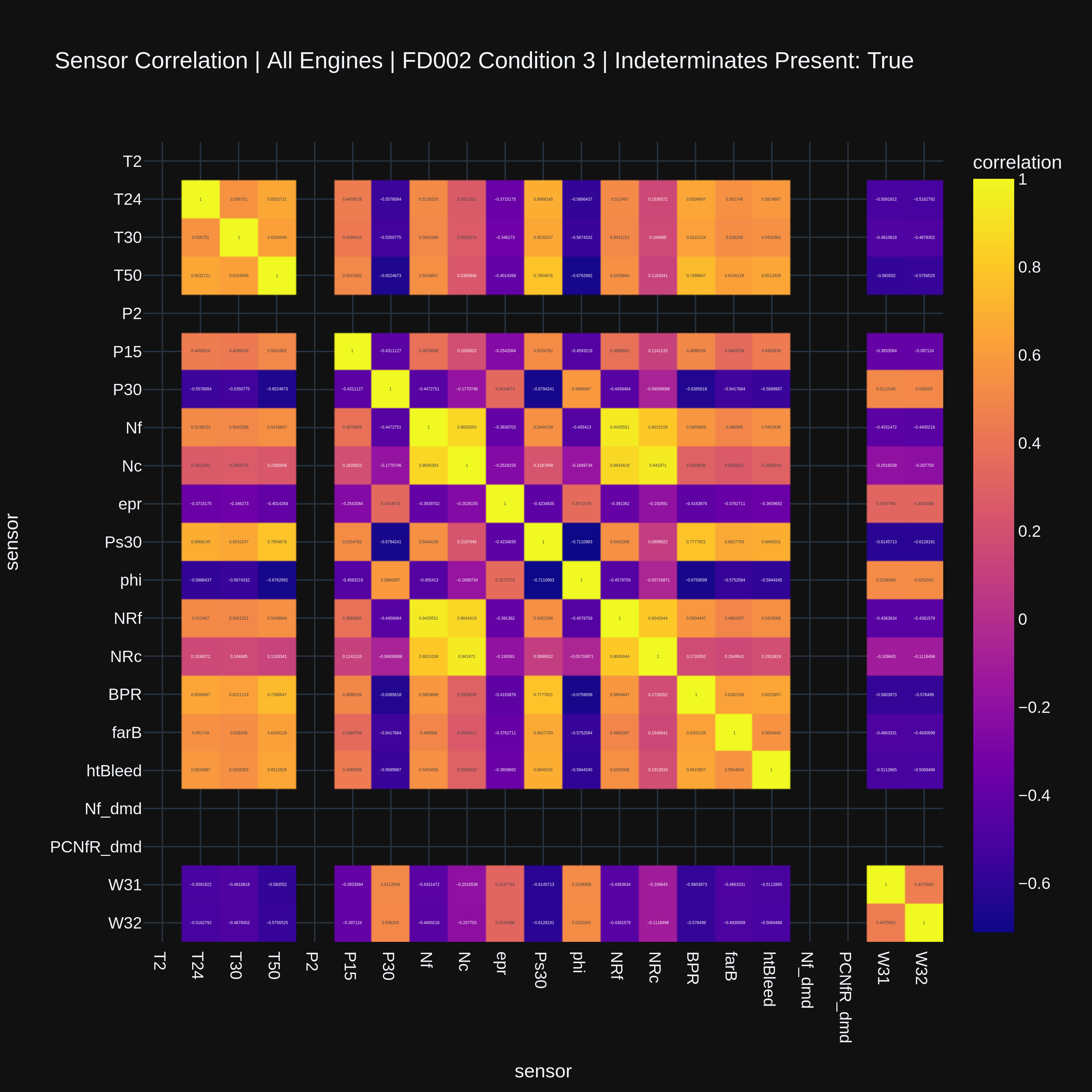
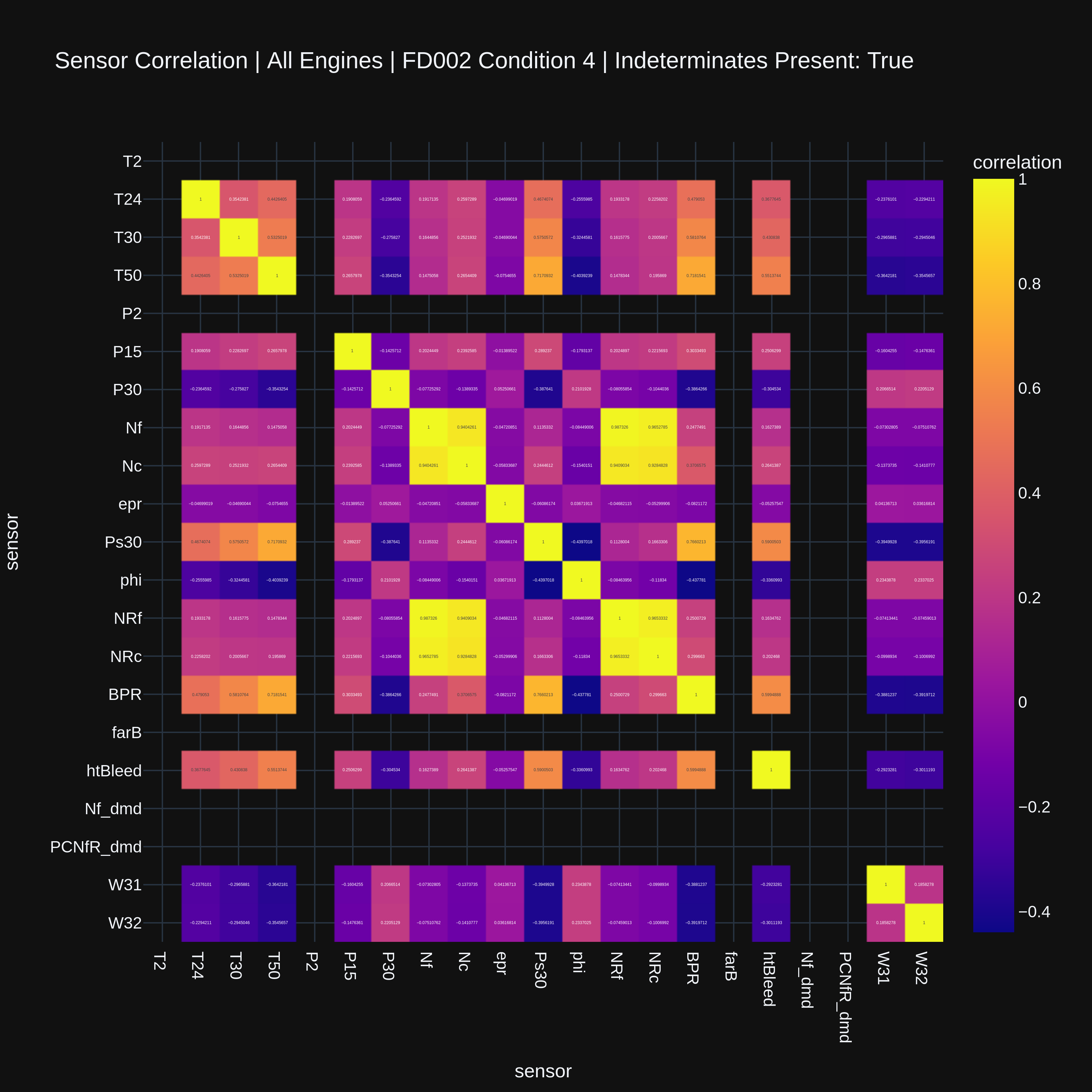
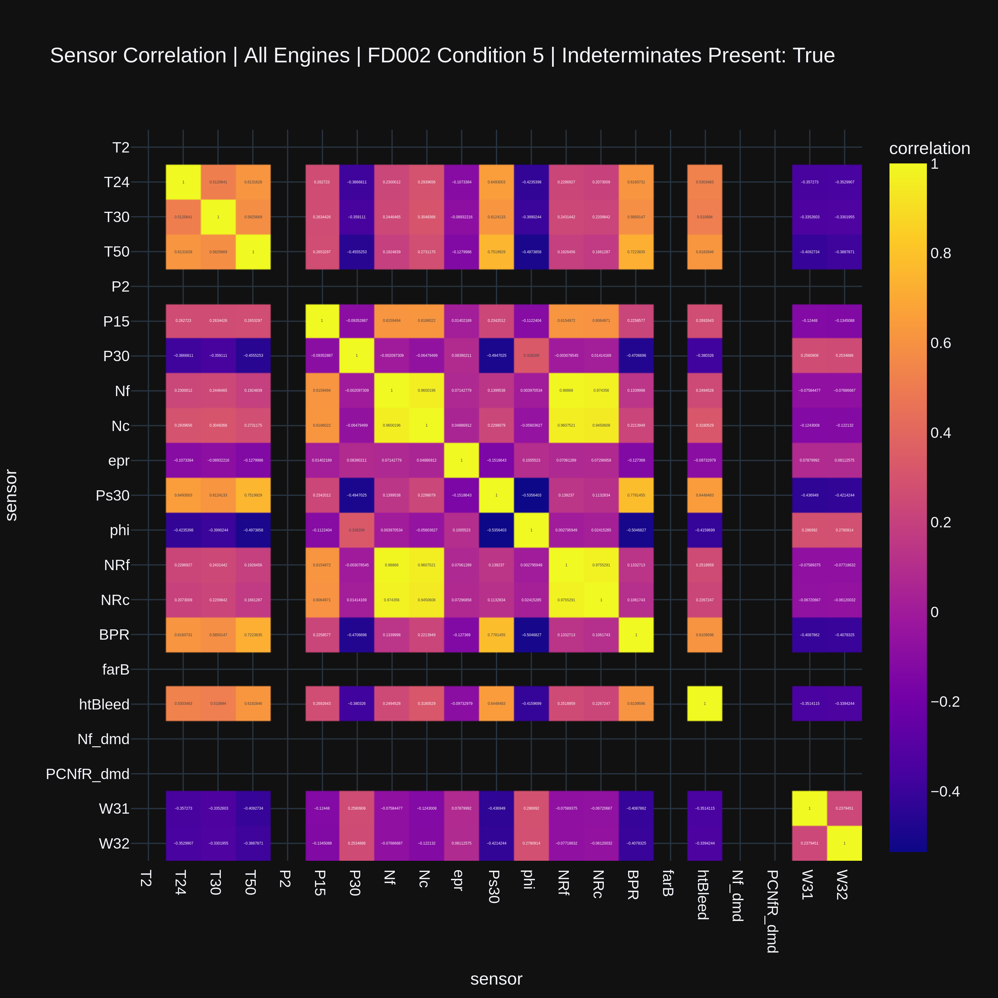
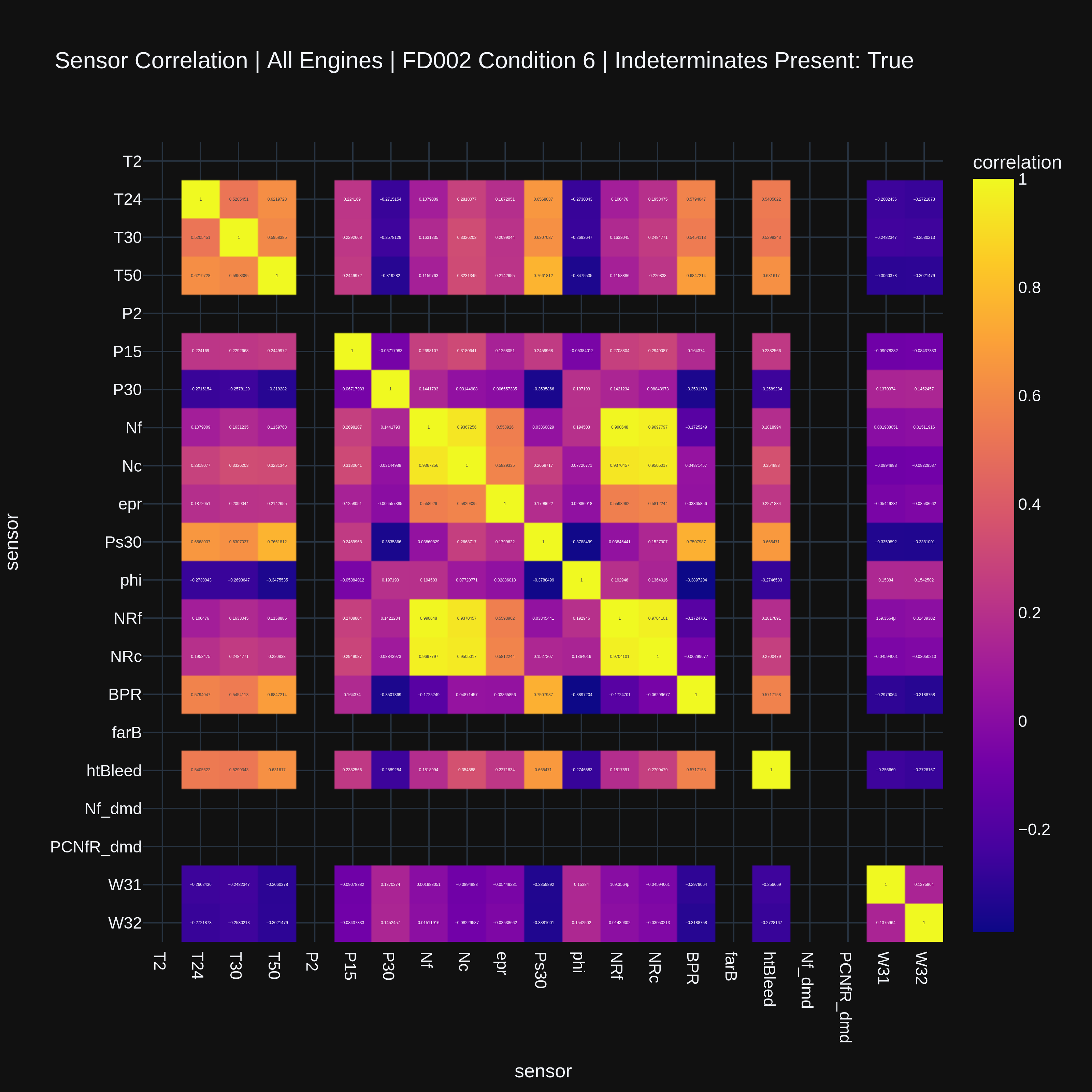
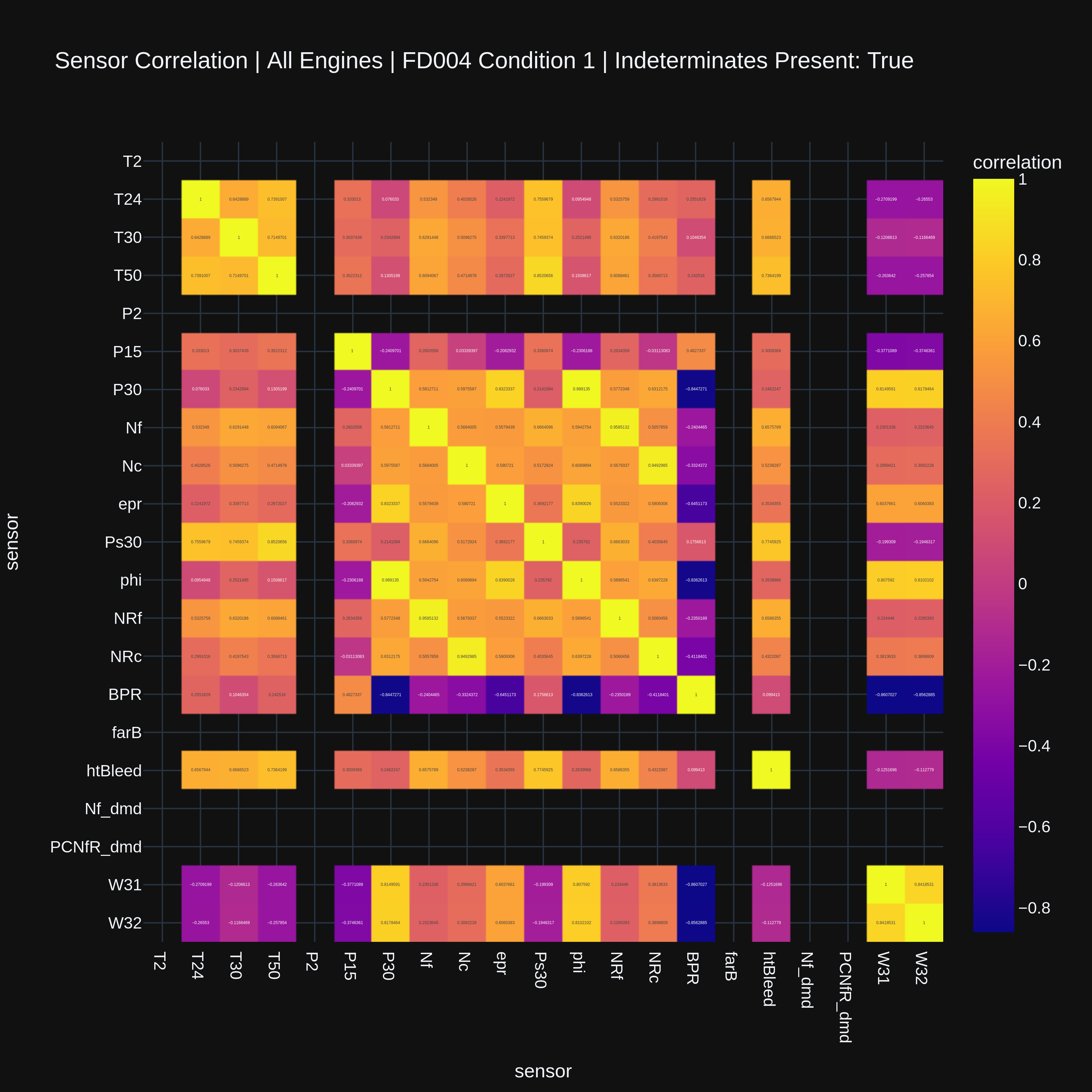
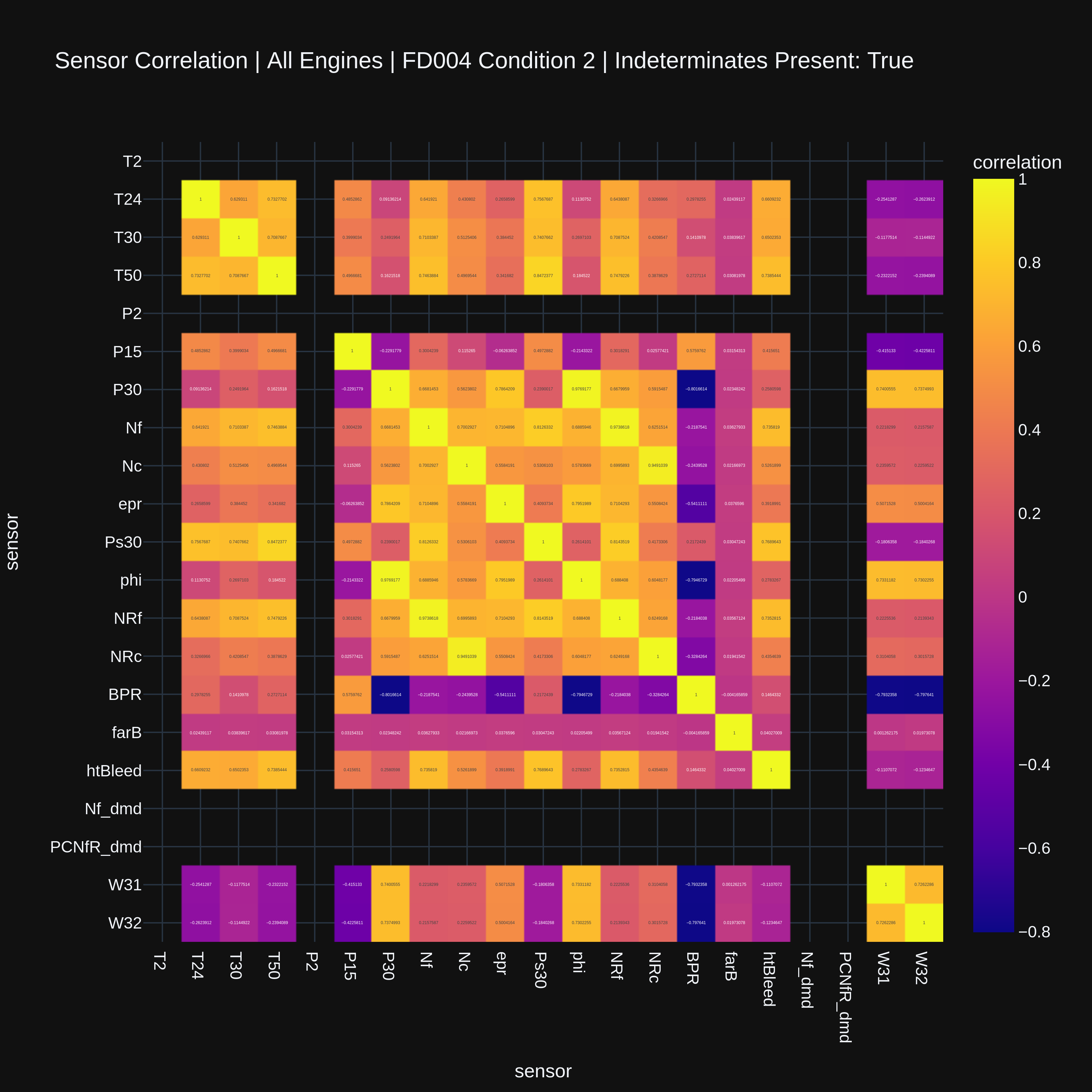
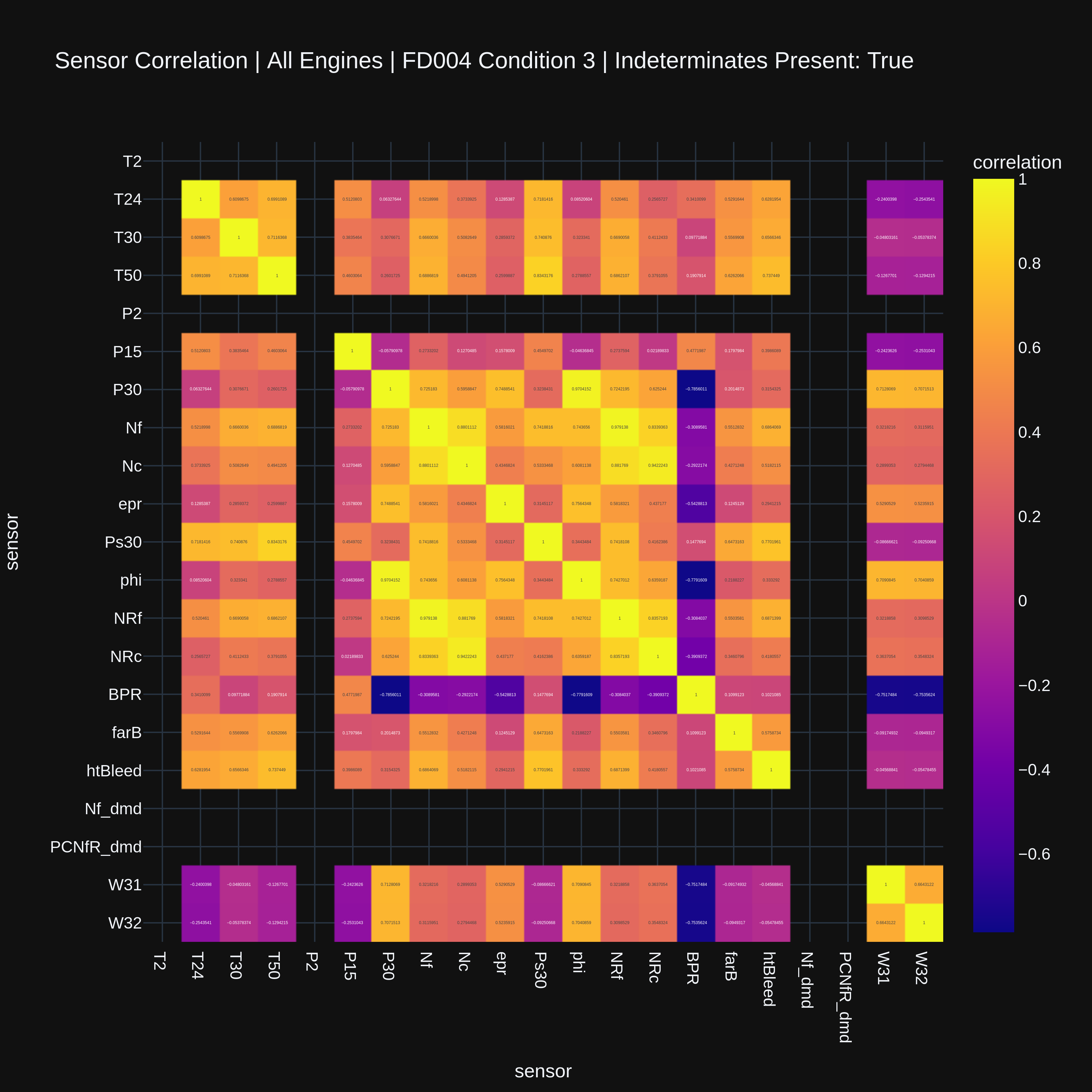
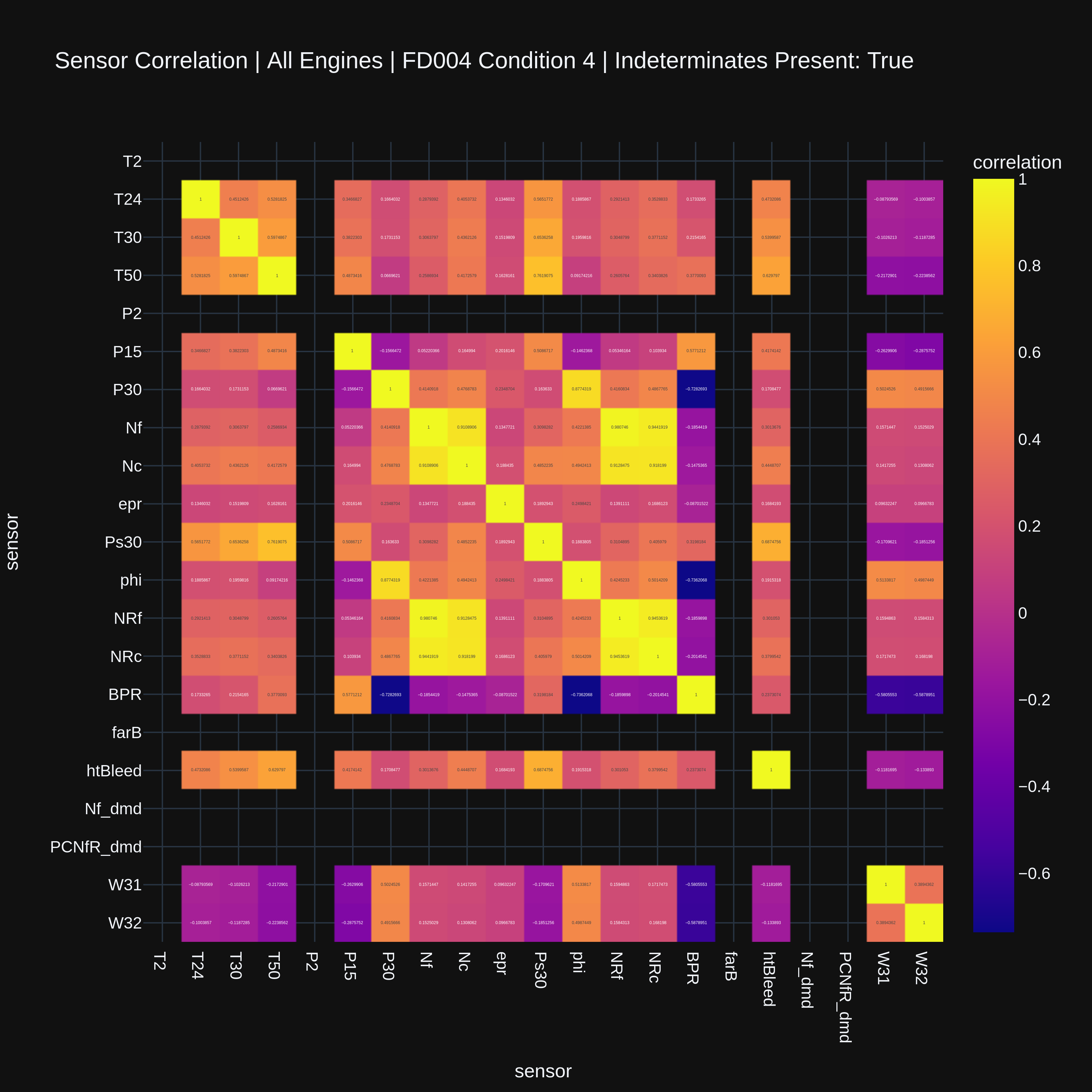
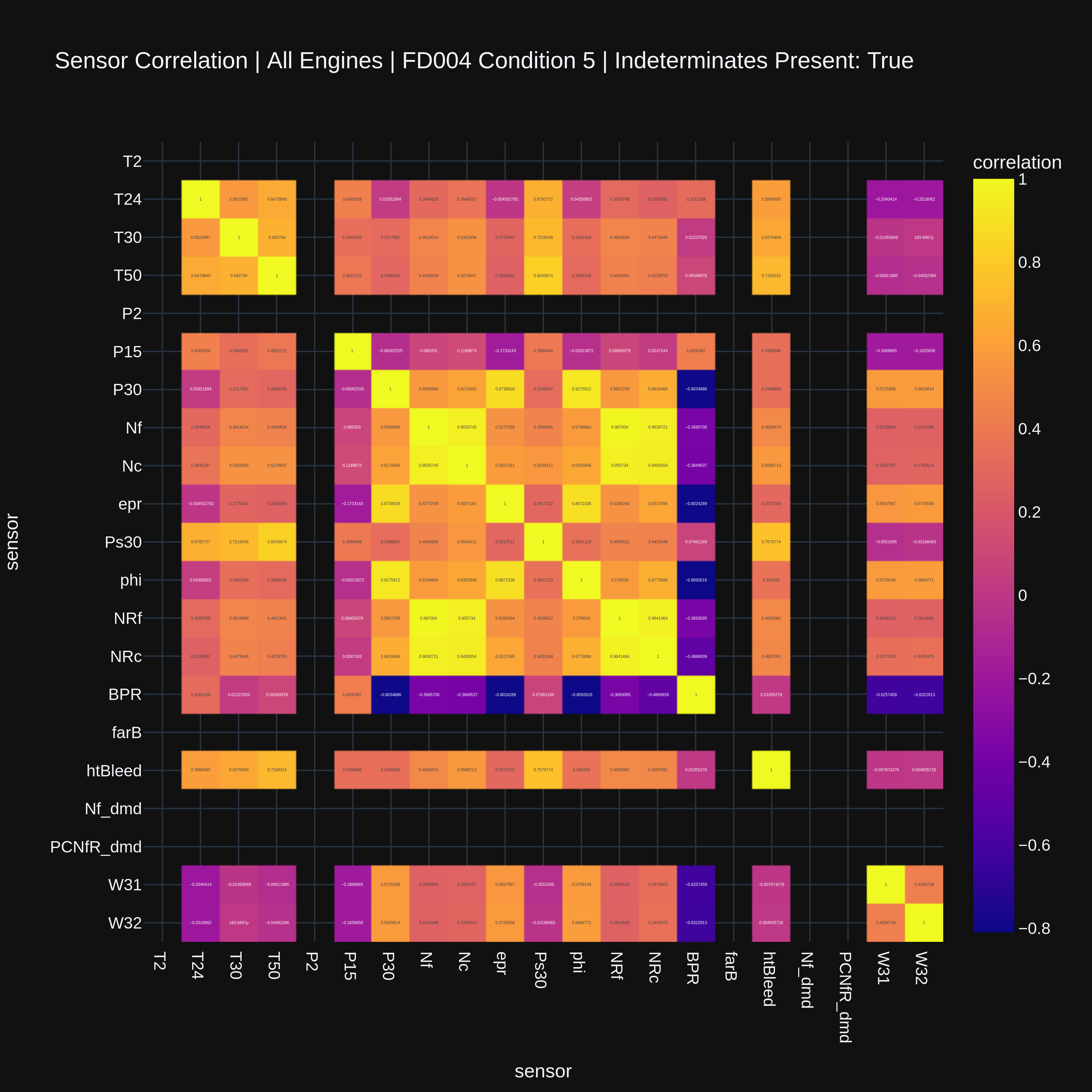
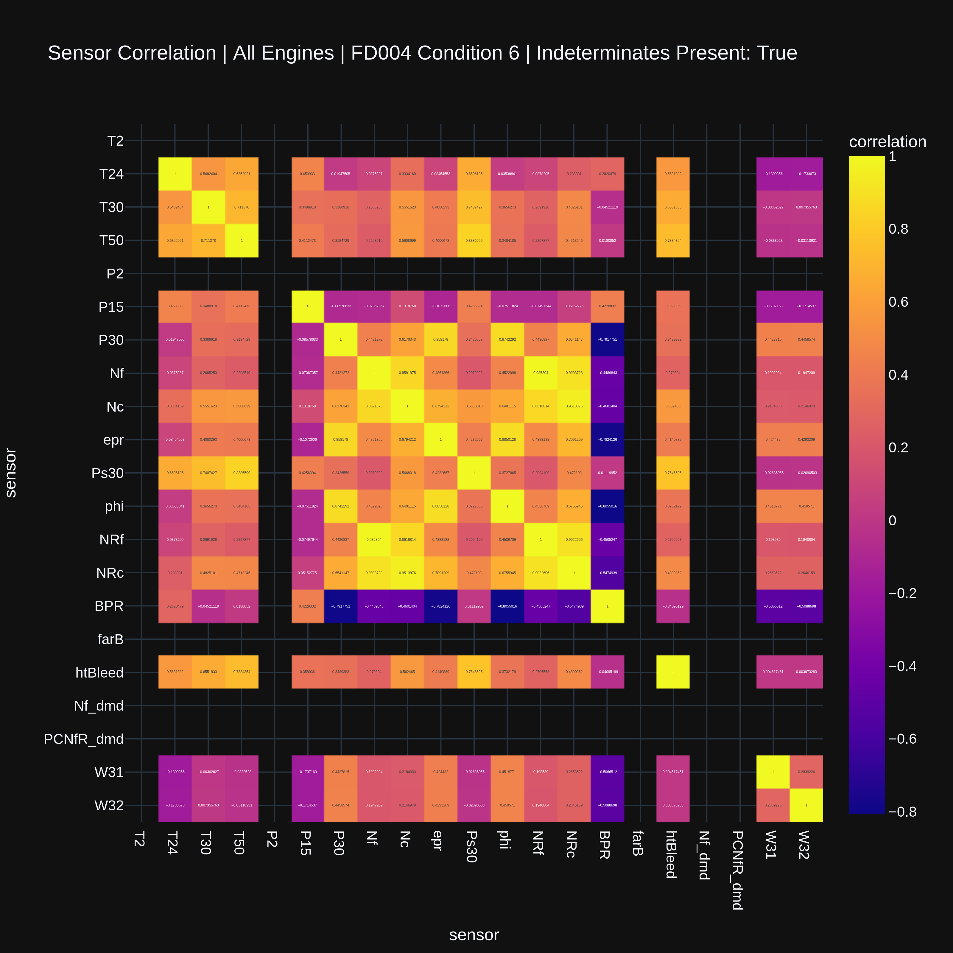
This leads me to believe that operating conditions act as a confounder for certain sensor relationships. This might be expected, since operating conditions vary with altitude, speed, and throttle resolver angle. I would expect indeterminate values if the dataset held those variables constant when some sensors depend on them to vary.

The Hypothesis

Here is where things started to get interesting for me. The jet engine’s fault mode isn’t included as an explicit feature in the relevant datasets FD003 and FD004. However, when visualizing the degradation graphs of the datasets using PCA across the sensors, I noticed that datasets FD003 and FD004 had separate clusters of faults present (Figure 4).

Figure 4

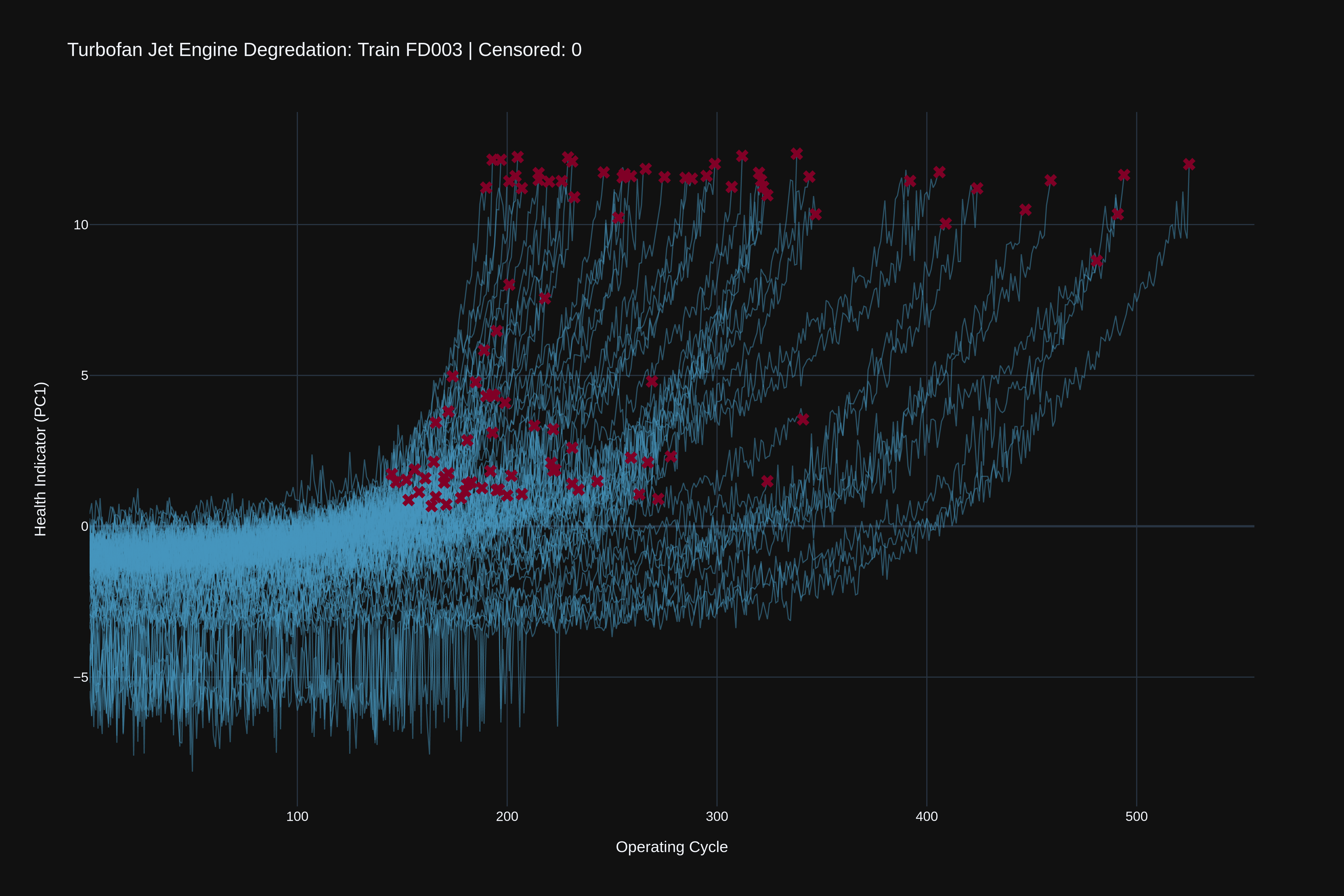
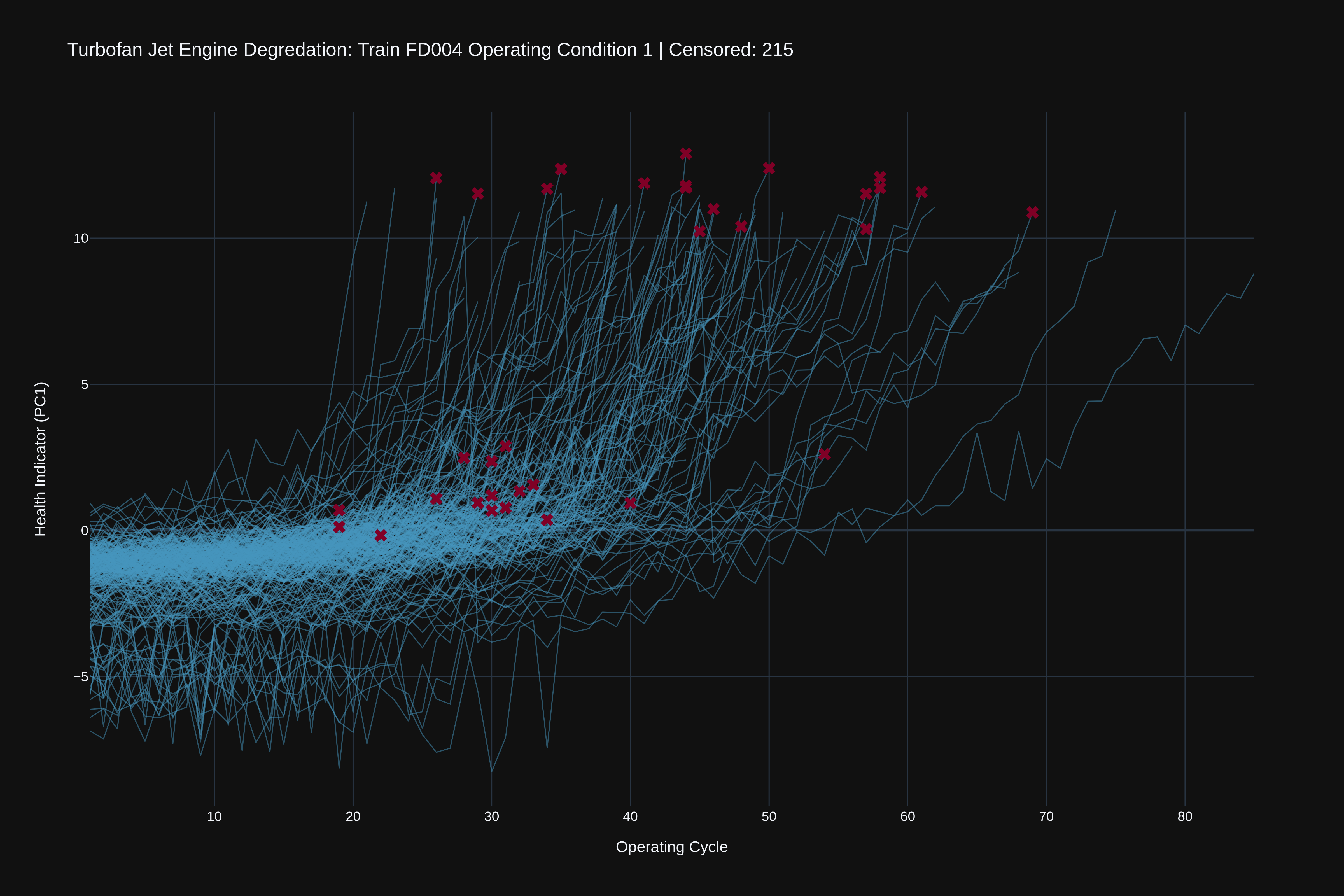
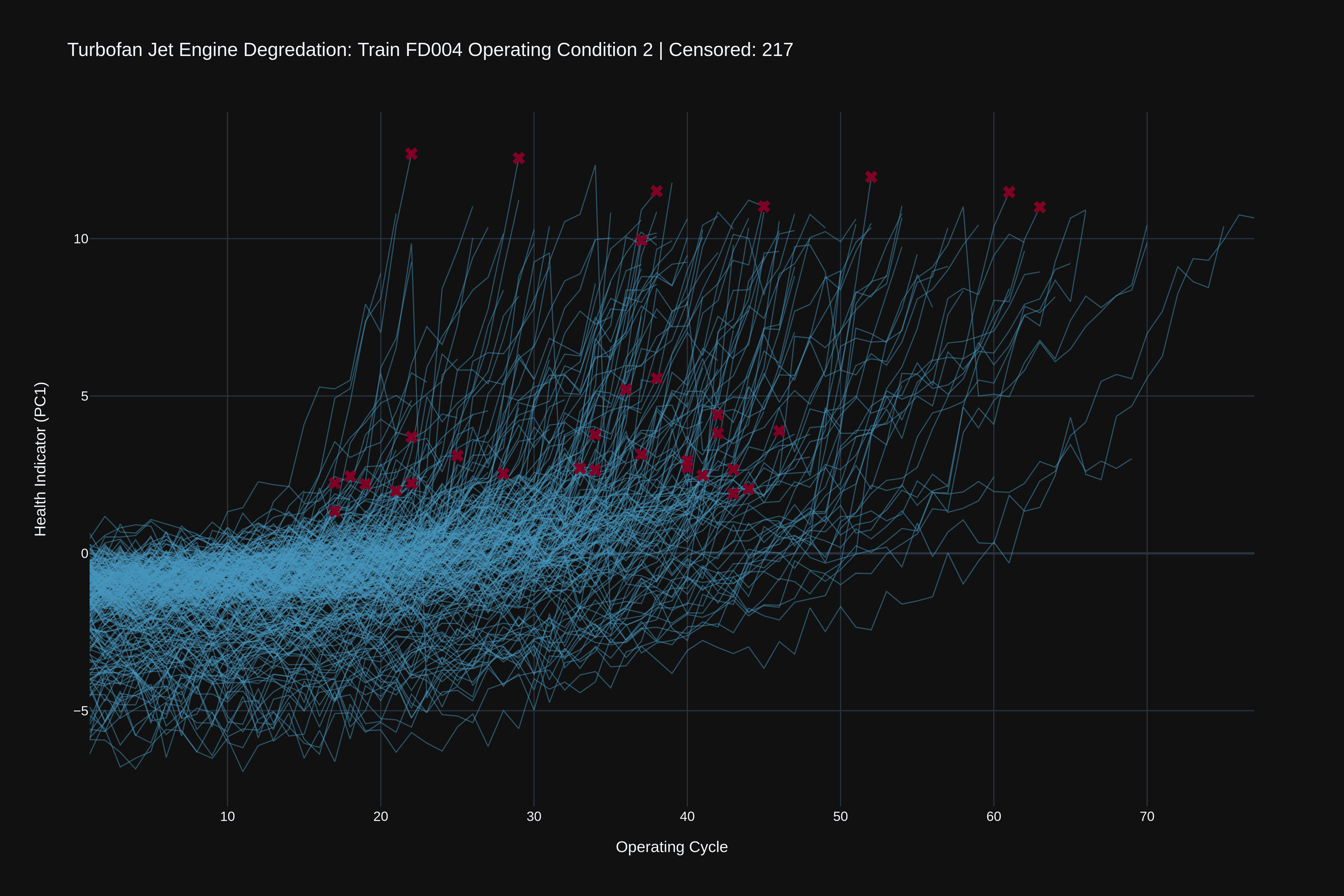
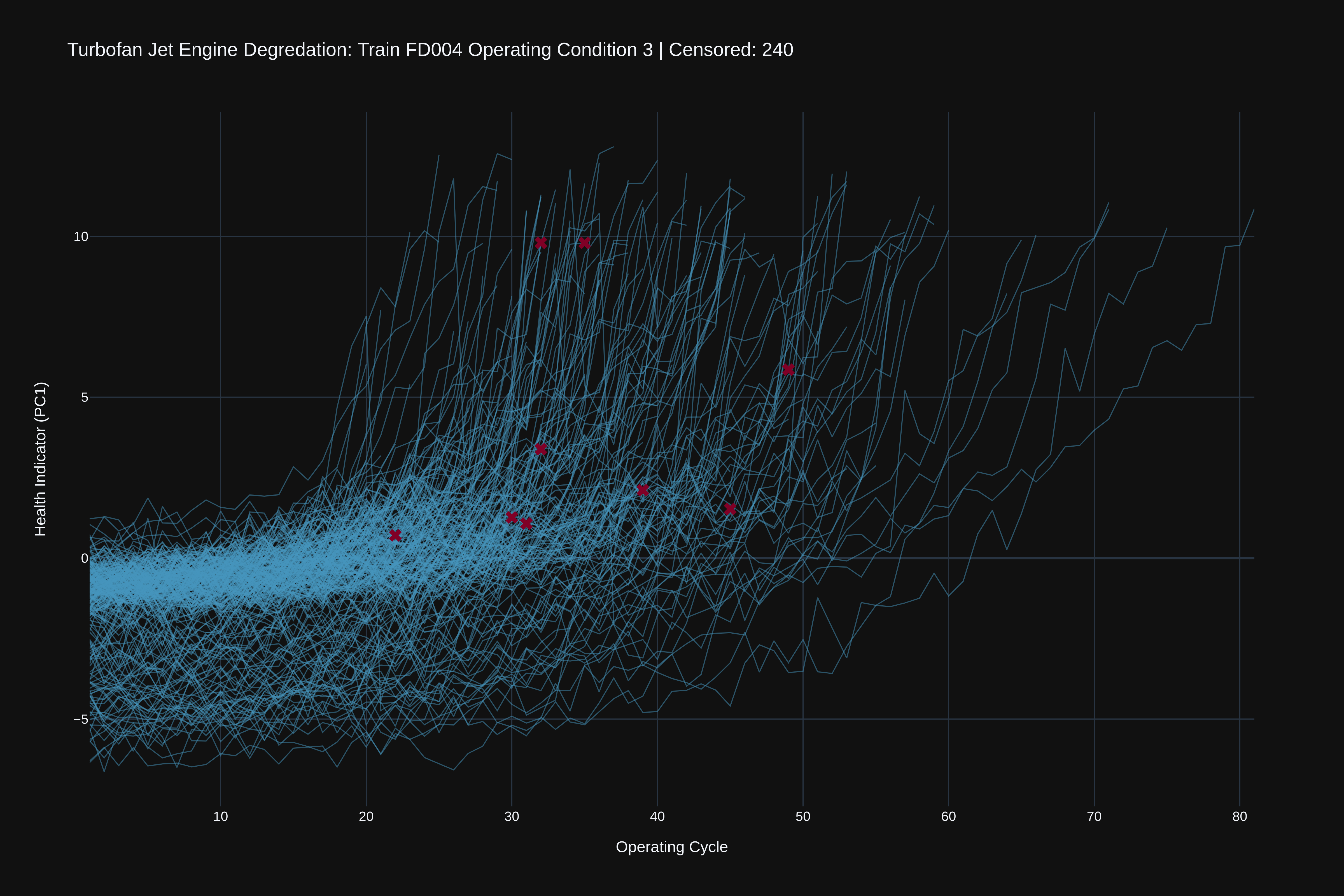
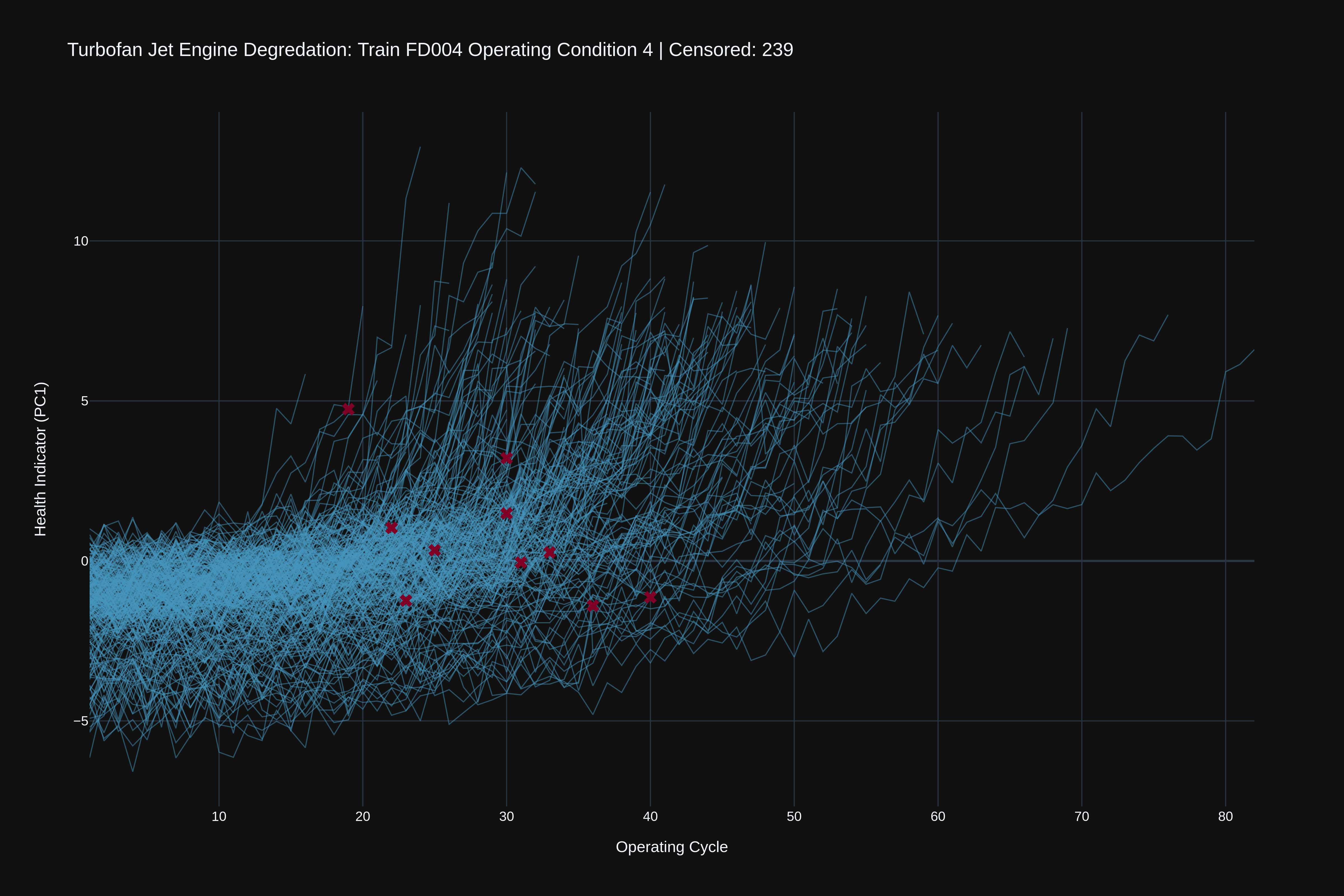
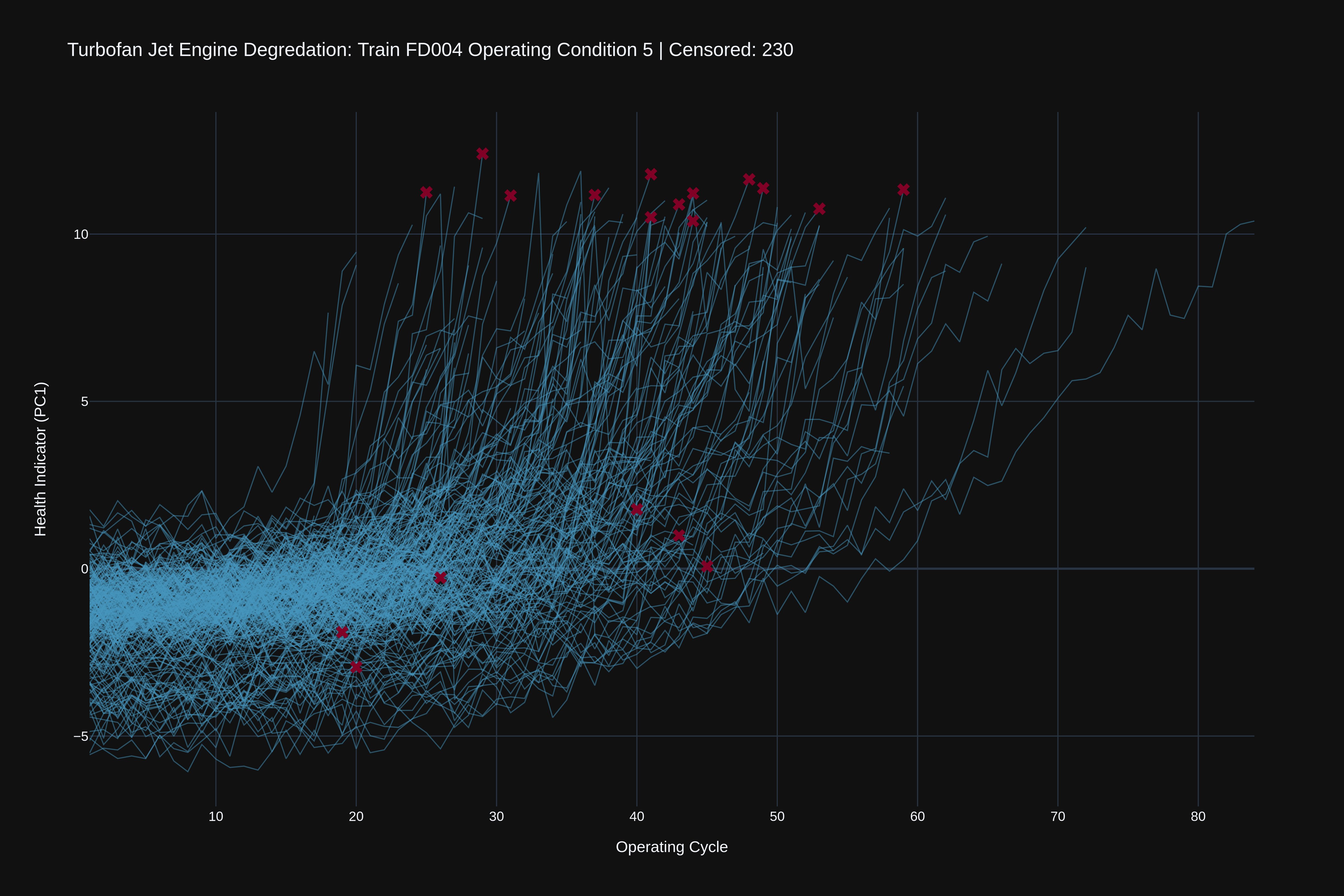
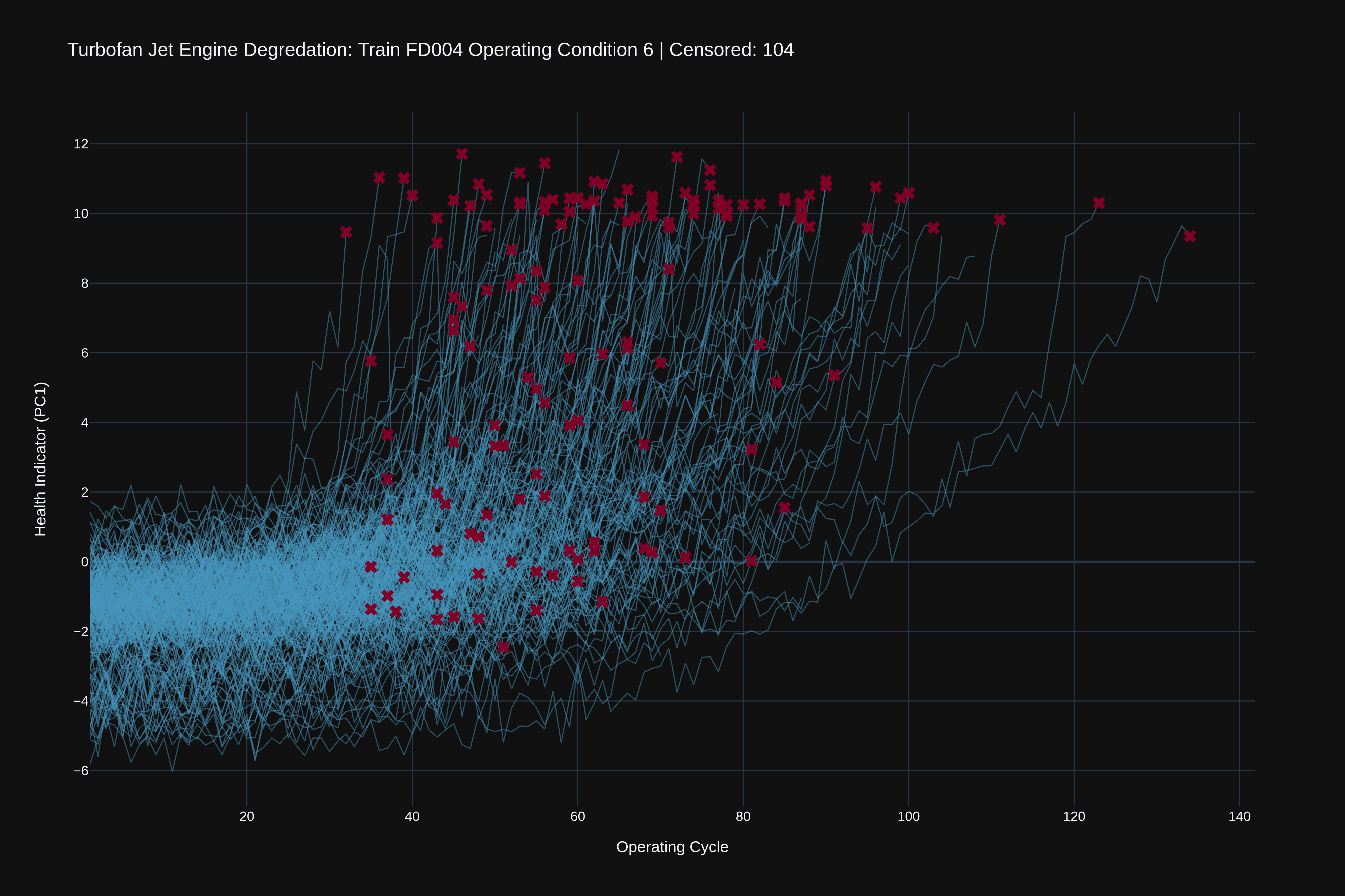
Principal component analysis (PCA) is a dimensionality reduction technique used to convert high-dimensional data into fewer dimensions called principal components. These principal components are ordered by the amount of variance they capture in the data, from greatest to least. The greatest variance component, PC1, was used to visualize the run-to-failure.

When I saw two distinct fault clusters in datasets with two fault modes, I thought a second principal component might represent this finding in the training data by capturing key information about the latent fault-mode feature. First, I fit PCA across the sensors with two principal components, and I visualized the degradation charts again. PC1 as the Y-axis, PC2 as the failure color artifact (Figure 5).

Figure 5

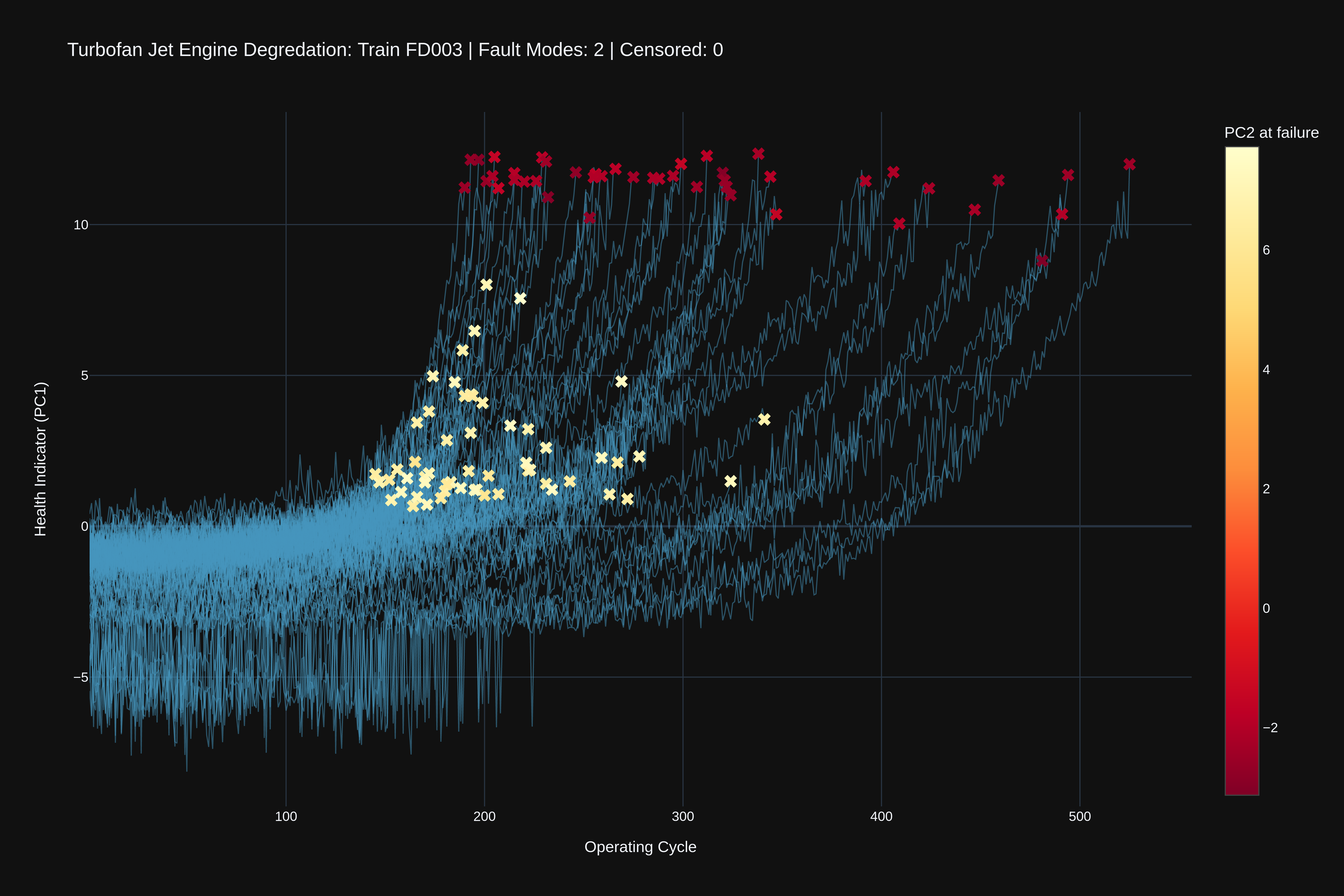
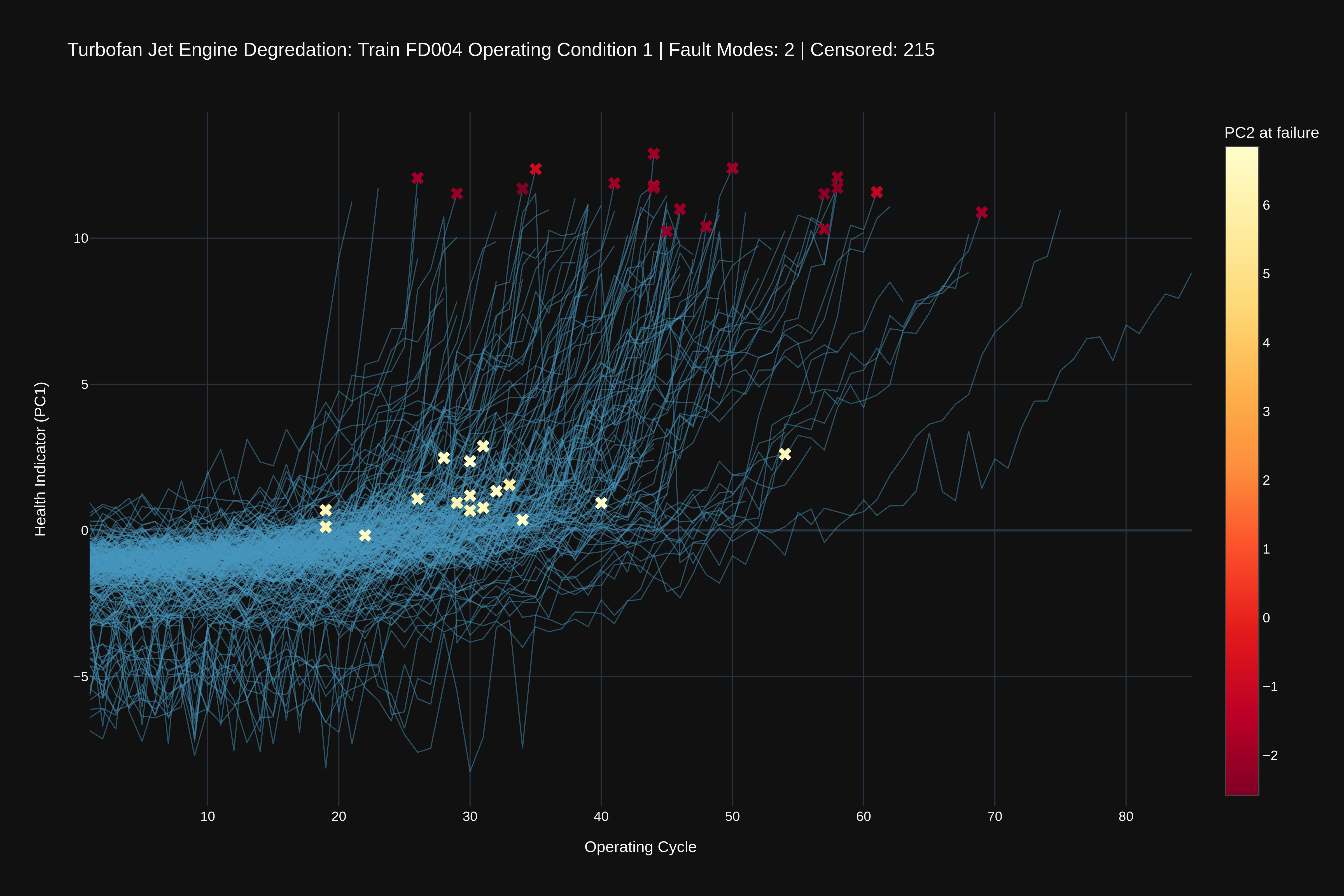
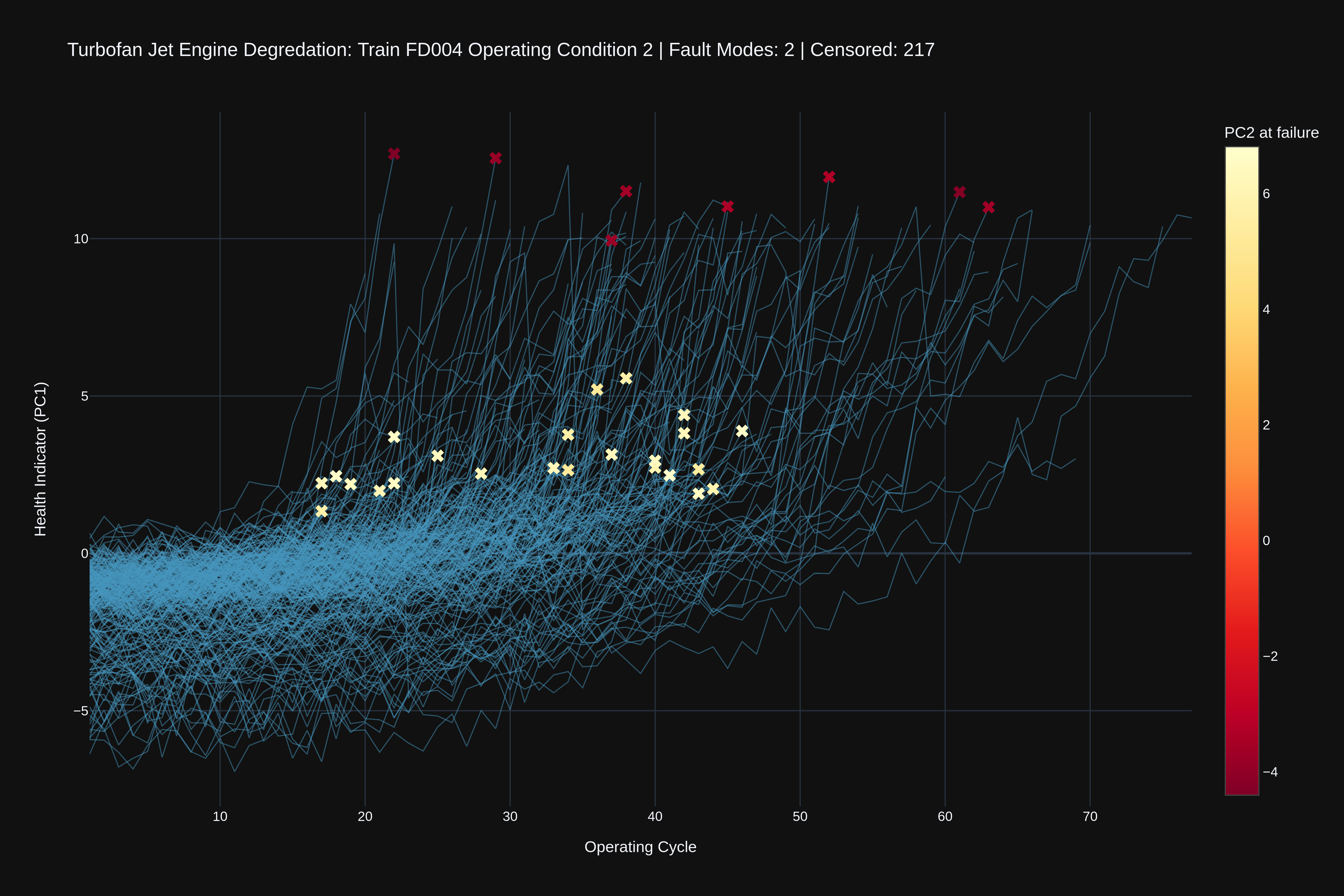
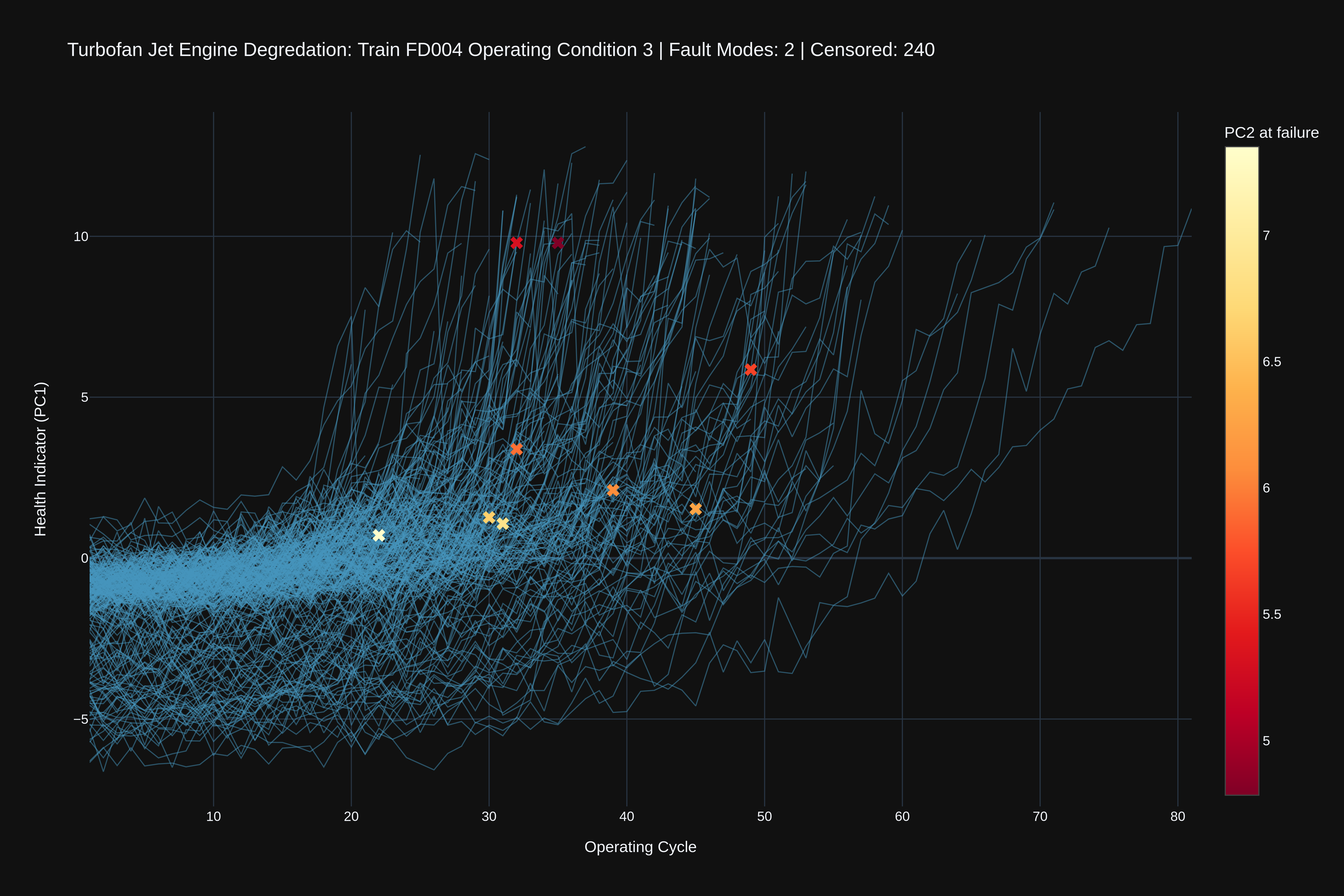
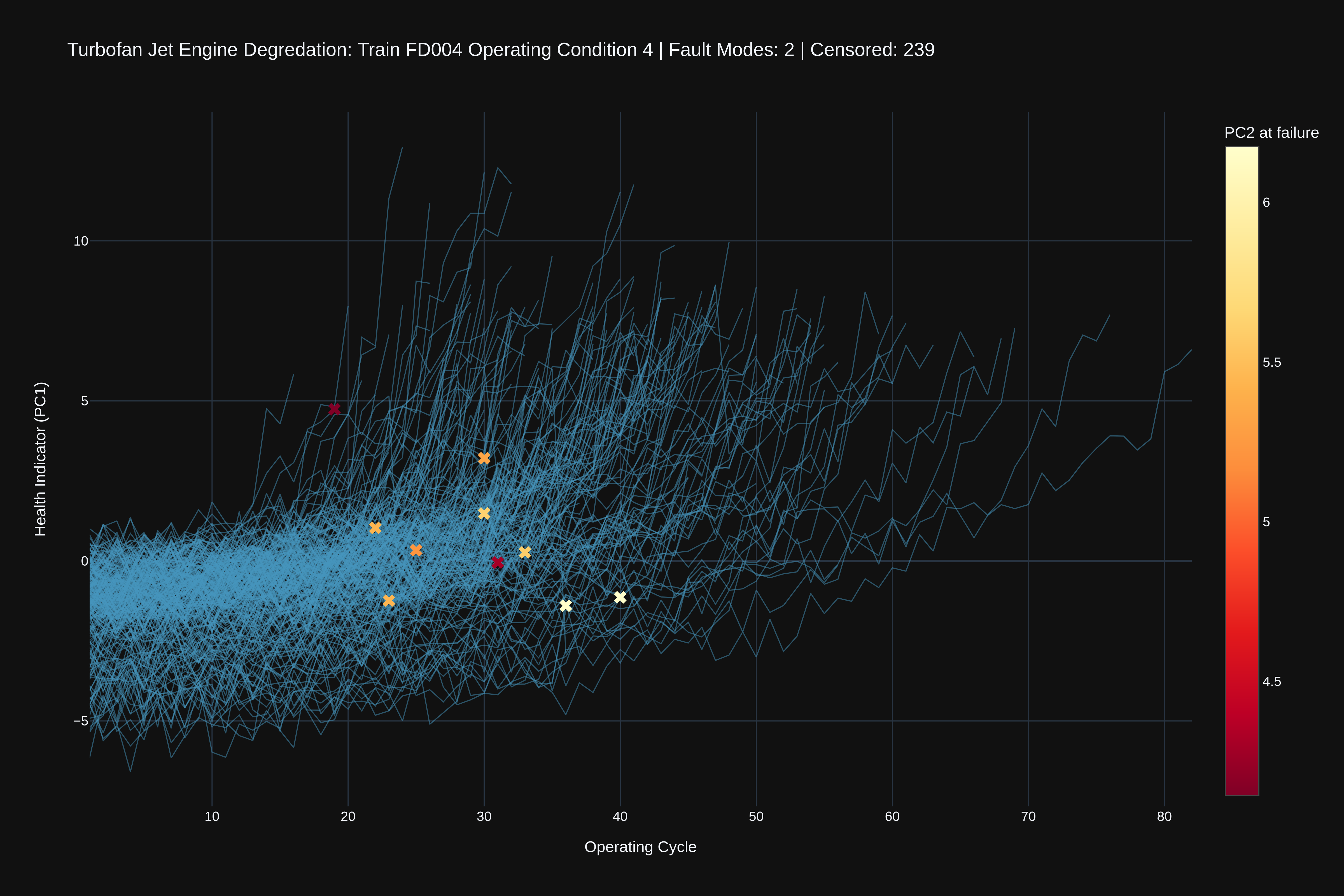
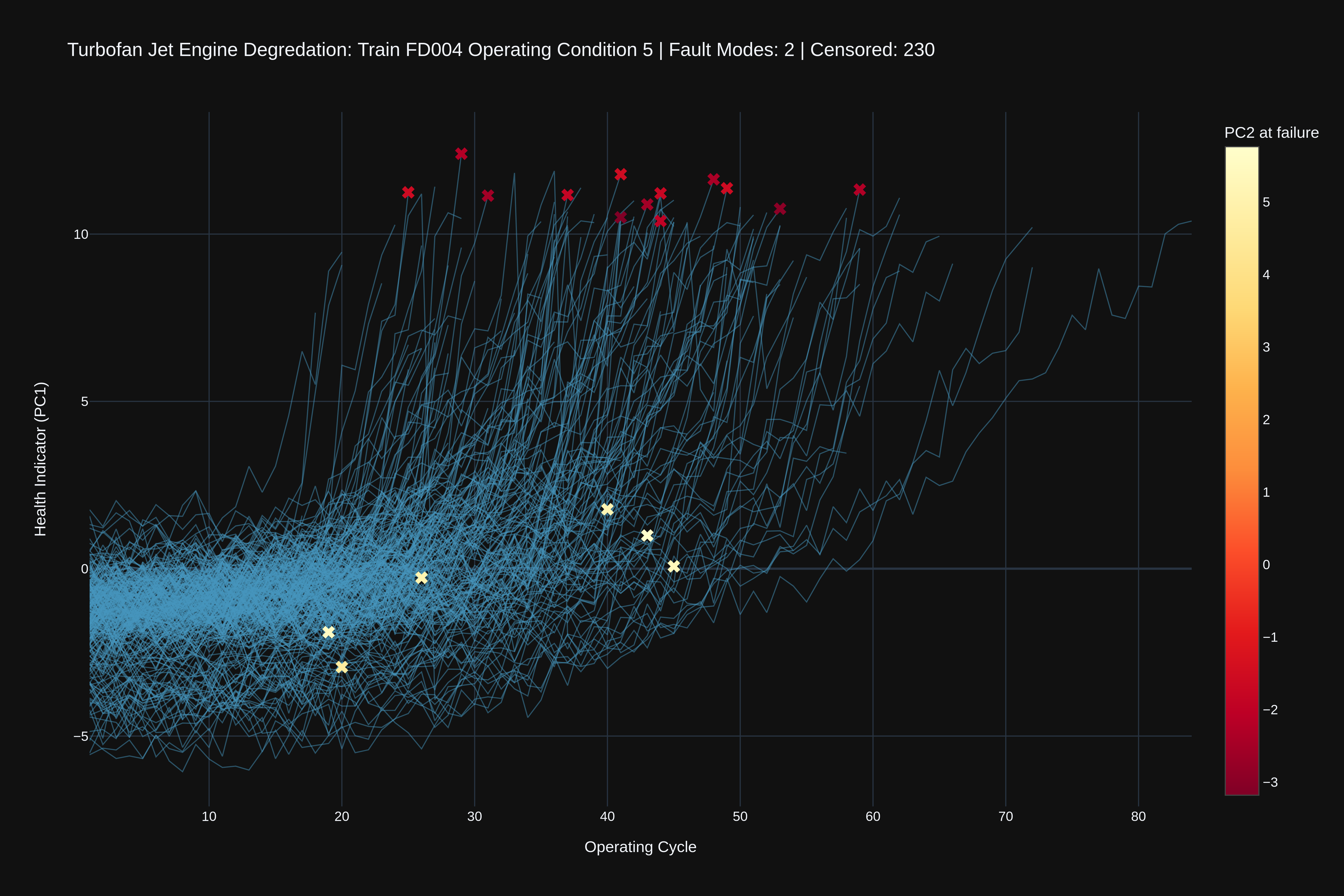
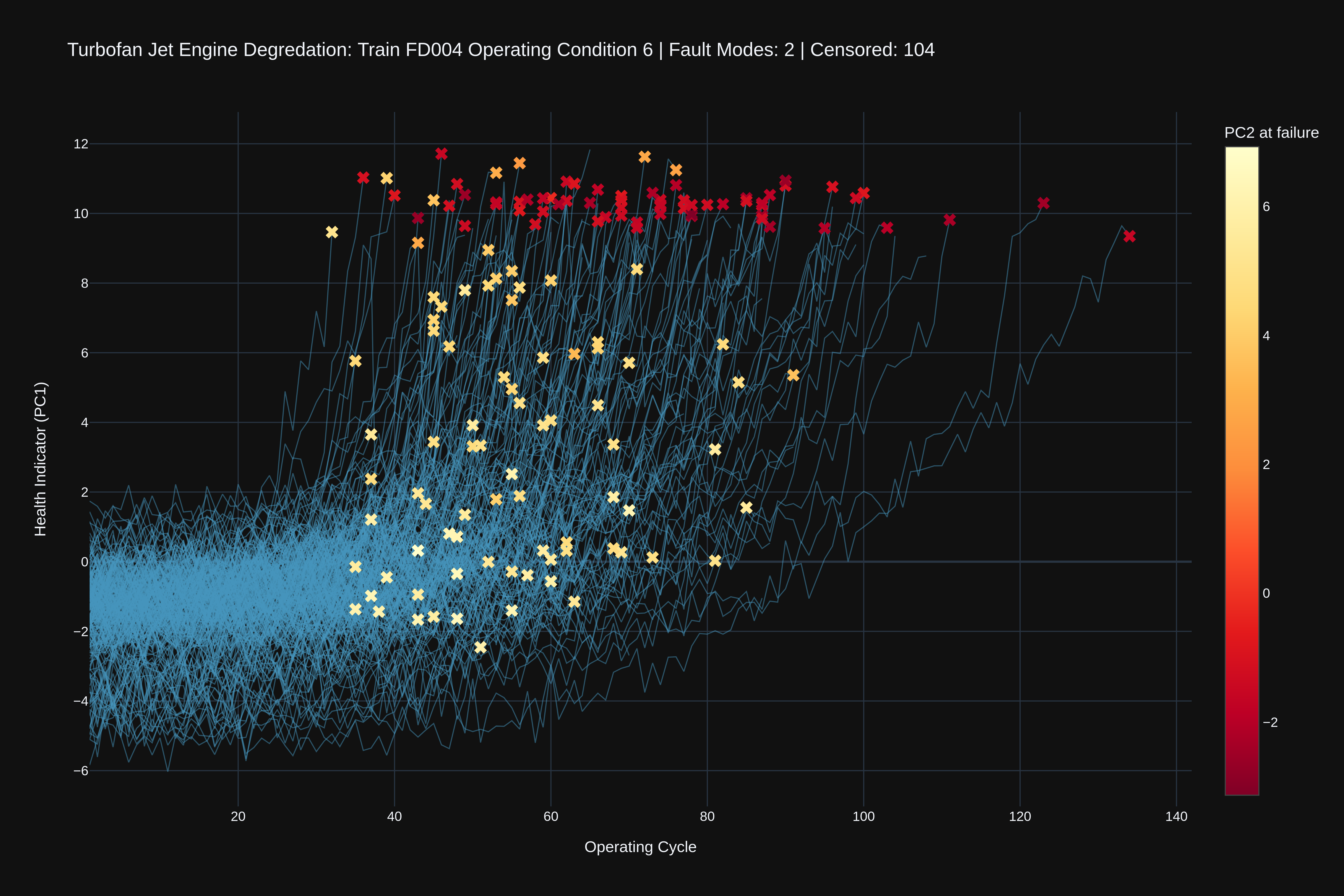
In the charts above, PC2’s color artifact shows a clear separation between clusters. Although it was not possible to definitively verify that PC2 represented the fault mode or closely related data, such as determining the causal contribution of each mode to the eventual failure or assessing the likelihood of bias toward either fault mode, the clear separation observed was sufficient to justify comparing model performance with and without PCA-derived training features.

My aim in this project was to evaluate the viability of PCA for latent feature modeling and feature engineering on this dataset, as well as to explore how these findings might generalize to other machine learning problems. While I can’t verify what variance PC2 is representing, I can verify performance disparities between models.

Experimentation

The original NASA C-MAPSS PHM08 Prognostics Challenge scored machine learning models based on how they performed on the test set with an asymmetric scoring function that punished late remaining-useful-life (RUL) predictions disproportionately. For each engine, let d = predicted RUL − true RUL. The total score is:

\[S = \sum_{i=1}^{N} s_i, \qquad s_i = \begin{cases} e^{-d_i/13} - 1, & d_i < 0 \\[4pt] e^{\,d_i/10} - 1, & d_i \ge 0 \end{cases}\]

Where $d_i = \widehat{\mathrm{RUL}}_i - \mathrm{RUL}_i$ is the predicted minus true remaining useful life, and $e$ is Euler’s number.

XGBoost Models trained for each dataset used an identical Optuna hyperparameter search over 300 trials:

def objective(trial): # Suggest a search space for XGBoost regression hyperparameters
params = {
"objective": metrics.cmapss_objective,
"n_estimators": trial.suggest_int("n_estimators", 100, 1000),
"n_jobs": -1,
"verbosity": 0,
"max_depth": trial.suggest_int("max_depth", 3, 10),
"learning_rate": trial.suggest_float("learning_rate", 0.001, 0.3, log=True),
"subsample": trial.suggest_float("subsample", 0.3, 1.0),
"colsample_bytree": trial.suggest_float("colsample_bytree", 0.3, 1.0),
"min_child_weight": trial.suggest_int("min_child_weight", 1, 10),
"gamma": trial.suggest_float("gamma", 0, 5),
"reg_alpha": trial.suggest_float("reg_alpha", 1e-8, 10.0, log=True),
"reg_lambda": trial.suggest_float("reg_lambda", 1e-8, 10.0, log=True),
"random_state": 42,
"device": "cuda",
}

    # Cross-validation setup to avoid overfitting
    groups = X_train.index  # engine id
    gkf = GroupKFold(n_splits=5)
    scores = []

    for train_idx, val_idx in gkf.split(X_train, y_train, groups=groups):
        X_tr, X_val = X_train.iloc[train_idx], X_train.iloc[val_idx]
        y_tr, y_val = y_train.iloc[train_idx], y_train.iloc[val_idx]

        model = XGBRegressor(**params)
        model.fit(X_tr, y_tr, eval_set=[(X_val, y_val)], verbose=10)

        preds = model.predict(X_val)
        score = metrics.cmapss_score(y_val, preds)
        scores.append(score)

    # Return the average validation metric to minimize
    return np.mean(scores)

Each hyperparameter search used a custom objective function designed to mimic the asymmetric loss function NASA uses for evaluating model performance:

def cmapss_objective(y_true, preds):
"""
Custom objective matching the CMAPSS asymmetric exponential penalty,
for use with the sklearn XGBRegressor API (not the native Booster API).
d = pred - true. Penalizes d > 0 (late prediction / RUL overestimate)
more steeply than d < 0.
"""
d = preds - y_true

    grad = np.where(d < 0, -(1 / 13) * np.exp(-d / 13), (1 / 10) * np.exp(d / 10))
    hess = np.where(d < 0, (1 / 169) * np.exp(-d / 13), (1 / 100) * np.exp(d / 10))

    return grad, hess

Feature engineering for this study involved extracting mean, standard deviation, and slope features from all datasets, while also incorporating operational condition labels specifically for FD002 and FD004, which contain multiple operating conditions. The final hyperparameters identified by Optuna’s search were applied to models trained with 25 random seeds, and the ensemble output was obtained by averaging the predictions of all base models.

PCA is fit once per dataset, on training data only, and then applied to train and test without refitting for FD003 and FD004. Because the test set never influences the fit, there’s no leakage, and a given PC2 value means the same thing in train and test.

For each subset (FD003 and FD004), fit_pca fits a StandardScaler and a 2-component PCA on that subset’s training frame, using only each engine’s last 60 cycles, where degradation dominates the variance. The scaler and PCA are then frozen.

def fit_pca(train_df, last_n=60, min_std=1e-3):
"""Fits one frozen scaler and 2-component PCA on training data.

    Standardizing gives each sensor unit variance, so none dominates
    by scale. PCA then finds orthogonal directions of maximum variance
    (eigenvectors of the covariance matrix): PC1 is the largest shared
    drift, PC2 the next largest direction perpendicular to it. Using
    late-life rows makes degradation, not noise, the main variance.
    Fitting once fixes the axes, so a PC2 value means the same thing
    for every engine and cycle.

    Args:
        train_df: Training frame. Engine id is the index, cycle is
            column 0, sensors are columns 4:25.
        last_n: Use each engine's final last_n cycles. None uses all.
        min_std: Drop near-constant sensors, since standardizing would
            inflate their noise.

    Returns:
        Tuple of (cols, scaler, pca).
    """
    cols = [c for c in train_df.columns[4:25] if train_df[c].std() > min_std]
    fit_df = train_df
    if last_n is not None:
        cyc = train_df.iloc[:, 0]
        last = cyc.groupby(level=0).transform("max")
        fit_df = train_df[cyc >= last - last_n]
    scaler = StandardScaler().fit(fit_df[cols])
    pca = PCA(n_components=2).fit(scaler.transform(fit_df[cols]))
    return cols, scaler, pca

add_pc2 only calls .transform(), so it standardizes the sensors with the training means and standard deviations and projects them onto the training PC2 axis. The same fitted objects are used for that subset’s train and test frames (scaler/pca for FD003, scaler1/pca1 for FD004).

def add_pc2(df, cols, scaler, pca):
"""Adds PC2 and its per-engine expanding mean as features.

    Projection is a dot product with a fixed unit vector, so it is
    cheap and identical for train and test. Fault mode is an
    engine-level trait, so a running mean of PC2 estimates it better
    than any single noisy row: noise shrinks roughly as 1/sqrt(n).
    The mean uses only current and past cycles, so it is causal.

    Args:
        df: Frame to transform (train or test), same layout as in
            fit_pca.
        cols: Sensor columns returned by fit_pca.
        scaler: Fitted StandardScaler from fit_pca.
        pca: Fitted PCA from fit_pca.

    Returns:
        out: Copy of df with 'pc2' inserted before the
        last two columns.
    """
    if df.equals(train3) or df.equals(test3):
        place = 1
    else:
        place = 2

    pc2 = pca.transform(scaler.transform(df[cols]))[:, 1]
    out = df.copy()
    out.insert(len(out.columns) - place, "pc2", pc2)
    return out

Evaluating the Impact of PC2 on FD003 and FD004: 25-Seed Ensemble Results Using Identical Hyperparameter Search

FD003

Seed	Score (No PC2)	RMSE (No PC2)	Score (PC2)	RMSE (PC2)
1	203.9	11.16	225.0	11.77
2	217.7	11.27	253.3	12.09
3	226.0	11.26	232.1	11.86
4	215.3	11.03	222.9	11.89
5	203.5	11.01	262.3	12.06
6	222.1	11.13	248.9	12.11
7	225.9	11.36	227.5	11.80
8	224.8	11.45	245.2	11.97
9	201.5	11.12	273.2	12.00
10	215.0	11.22	228.2	11.84
11	211.8	11.02	222.8	11.73
12	231.7	11.50	240.2	11.71
13	226.5	11.20	227.8	11.79
14	236.0	11.43	215.5	11.74
15	186.8	10.91	220.9	11.82
16	194.0	10.92	212.5	11.52
17	220.2	11.46	229.7	11.67
18	224.5	11.37	247.9	12.25
19	249.5	11.42	236.3	11.91
20	220.2	11.25	244.2	11.96
21	204.0	11.09	241.7	11.87
22	212.6	11.42	222.9	11.73
23	211.5	11.08	217.9	11.69
24	206.2	11.07	227.3	11.65
25	220.5	11.26	224.4	11.64
mean	216.5	11.22	234.0	11.84
best	186.8	10.91	212.5	11.52
worst	249.5	11.50	273.2	12.25
bag	202.4	11.19	224.2	11.80

FD004

Seed	Score (No PC2)	RMSE (No PC2)	Score (PC2)	RMSE (PC2)
1	3276.2	23.35	3119.5	23.19
2	3266.2	23.44	3182.0	23.27
3	3256.7	23.40	3155.5	23.35
4	3338.0	23.38	3149.3	23.21
5	3489.8	23.71	3154.5	23.24
6	3480.3	23.79	3141.6	23.04
7	3401.2	23.55	3133.9	23.40
8	3447.2	23.67	3234.6	23.46
9	3286.5	23.59	3329.6	23.40
10	3336.0	23.74	3327.6	23.35
11	3261.9	23.45	3250.2	23.40
12	3230.5	23.42	3336.0	23.56
13	3453.7	23.61	3058.1	23.07
14	3568.6	23.61	3079.9	23.25
15	3302.0	23.60	3326.2	23.40
16	3477.8	23.65	3414.9	23.41
17	3223.1	23.43	3118.2	23.10
18	3121.7	23.42	3104.7	23.24
19	3219.0	23.43	3318.9	23.36
20	3272.9	23.52	3135.1	23.25
21	3368.9	23.53	3223.7	23.27
22	3364.4	23.50	3212.6	23.35
23	3198.9	23.45	3235.0	23.16
24	3137.7	23.27	3133.7	23.20
25	3360.2	23.64	3083.1	23.34
mean	3325.6	23.53	3198.3	23.29
best	3121.7	23.27	3058.1	23.04
worst	3568.6	23.79	3414.9	23.56
bag	3262.12	23.41	3145.3	23.17

Both model ensembles, with and without PC2 features, were trained using the same hyperparameters. These Hyperparameters were provided by the initial search over the frames without PC2 features.

FD003: Adding PC2 degraded performance, increasing the mean S-score from 216.5 to 234.0 (+8.1%) and mean RMSE from 11.22 to 11.84 (+5.5%). This suggests PC2 provides little useful signal for FD003 and may introduce noise that harms predictive performance.

FD004: Adding PC2 improved performance, reducing the mean S-score from 3325.6 to 3198.3 (−3.8%) and mean RMSE from 23.53 to 23.29 (−1.0%). The improvement is modest for RMSE but more pronounced for the asymmetric S-score, suggesting PC2 provides useful information for FD004.

Final Thoughts

Results

Model	JetBoost GBM (S-score)	RMSE
FD001	193	11.45
FD002	3894	22.94
FD003	202	11.19
FD004	3145	23.17

JetBoost GBM models were evaluated on the labeled observations in the NASA C-MAPSS test set. Rows with missing RUL values were excluded, leaving the final labeled observation for each test engine. Predictions were evaluated against the original, uncapped RUL labels.

def cmapss_score(y_true, y_pred):
d = np.asarray(y_pred) - np.asarray(y_true)
return np.sum(np.where(d < 0, np.exp(-d/13) - 1, np.exp(d/10) - 1))

scoreable_test = test.dropna(subset=["RUL"])
X_test = scoreable_test.drop(columns=["RUL"])
y_test = scoreable_test["RUL"]
preds = GBM.predict(X_test)

# NASA score

score = cmapss_score(y_test, preds)

# RMSE in cycles

rmse = root_mean_squared_error(y_test, preds)

print("NASA S Score:", score)
print("RMSE:", rmse)

No additional RUL capping was applied during evaluation. Consequently, the reported metrics reflect predictions scored against the original test labels, including RUL values greater than 125 cycles.

PCA Features?

Although the inclusion of PCA-derived features appeared to add noise for FD003 and provided only modest improvement for FD004, this might be due to the possibility that fault modes are already encoded in the sensor data. In cases like these, engineered features from PCA may not necessarily contribute additional useful information if the main sources of variation are already captured by the original features.

However, PCA features might still be helpful in other machine learning tasks. For example, if less is known about the underlying structure of the data or the relationships between features and labels are more complex, PCA could potentially uncover latent patterns that are not immediately apparent in the original variables. In this case, the second principal component seemed to correspond to separate clusters that might relate to different fault modes, suggesting that, without prior knowledge of these modes, PCA might still capture meaningful variance. As such, while the results for this specific task were not impressive, PCA-derived features could be beneficial in other situations, especially where the data structure is less well understood or more complex.

Overall, the PCA features were a small win on FD004 and a wash on FD003, not the breakthrough I was hoping for. If you try something similar on your own data, I’d like to hear whether it does anything for you. Thanks for reading!

Acknowledgements

I gratefully acknowledge the NASA Prognostics Center of Excellence (PCoE) for making the Commercial Modular Aero-Propulsion System Simulation (NASA C-MAPSS) dataset publicly available for this workshop.